of Skin Color Cue in Face Detection Applications

Fig. 1

Block diagram of a generic face recognition system

The purpose of face detection is to process still images or image sequences to find the location(s) and the size(s) of any faces in them [31]. Although face detection is a trivial task for humans, it is very challenging to build a stable automatic solution since face patterns significantly vary under different facial poses/expressions, occlusion conditions, and imaging condition (e.g. illumination condition, sensor characteristics). Various face detection algorithms have been proposed [31, 75, 79], but achieving highly accurate detection performance while maintaining reasonable computational costs still remains to be a challenging issue.

In general, existing face detection methods are grouped into the two main categories [31]: (i) feature-based approach, (ii) image-based approach. In feature-based approach [33, 48, 54, 58, 72], explicit face features (e.g. eyes, mouth, nose and face contour) are extracted, then relationships between them (such as geometric and morphologic relationships) are used to determine the existence of the face. For instance, Sobottka and Pitas [72] proposed a two-stage face detection framework to locate face regions in color image. The first stage is dedicated to segment face-like regions by skin color analysis using hue and saturation information in HSV colorspace, followed by shape analysis using ellipse fitting. Afterwards, grayscale information of detected face-like regions are examined to verify them by locating eye and mouth features. Extending the feature-based approach, Hsu et al. [33] localized face candidates from color image using skin color cue in YCbCr colorspace and constructed eye, mouth, face boundary maps to verify each face candidate. The methods in this category are advantageous due to their relatively simple implementation and high detection accuracy in uncluttered backgrounds. In particular, skin color cue is exceptionally popular and successful in feature-based approach due to its simplicity and high discrimination power. Some of these methods remain very popular nowadays in certain applications such as mobile phone applications. However, they tend to have difficulties in dealing with challenging imaging conditions such as varying illumination and complex background, as well as low resolution images containing multiple faces.

Alternatively, image-based approach [9, 13, 67, 80] uses machine learning techniques to capture unique and implicit face features, treating the face detection problem as a binary classification problem to discriminate between face and non-face. Often, methods in this category require tremendous amount of time and training data to construct a stable face detection system. However, in recent years, the rapid advancement in digital data storage and digital computing resources has made the image-based approaches feasible to many real-life applications and they become extremely popular due to their enhanced robustness and superior performance against challenging conditions compared to feature-based approaches.

One of the most representative works in image-based approach is the Viola-Jones’s face detection framework [67], a Haar-like feature based frontal face detection system for grayscale images. The Haar-like feature represents the differences in grayscale between two or more adjacent rectangular regions in the image, characterizing local texture information. In Viola-Jones framework, AdaBoost learning algorithm is used to handle following three fundamental problems: (i) learning effective features from a large Haar-like feature set, (ii) constructing weak classifiers, each of which is based on one of the selected features, (iii) boosting the weak classifiers to construct a strong classifier. The authors applied the integral image technique for fast computation of Haar-like features under varying scale and location, achieving real-time operation¹. However, the simplicity of Haar-like features in Viola-Jones face detector causes limited performance under many complications, such as illumination variation. More recent approaches address this problem by using an alternative texture feature called Local Binary Pattern (LBP), which is introduced by Ojala et al. [50] to offer enhanced discriminative power and tolerance towards illumination variation. 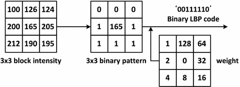The LBP descriptor encodes the relative gray value differences from a $3\times 3$ neighborhood of an image patch as demonstrated in Fig. 2. By taking the center pixel as a threshold value, every neighboring pixel is compared against the threshold to produce a 8-bit string, and then binary string is converted to decimal label according to assigned weights. Many variants of LBP features are considered thereafter, such as LBP Histogram [26], Improved Local Binary Pattern (ILBP) [35], Multi-Block LBP (MB-LBP) [80], and Co-occurrence of LBP (CoLBP) [47].

Fig. 2

Example of basic LBP feature computation

Although considerable progress has been made in aforementioned image-based face detection methodologies, the main emphasis has been placed on exploiting various grayscale texture patterns. A few recent researches [12, 25] have shown that color cue could provide complementary information to further enhance the performance of image-based approaches. Specifically, color information could potentially enhance the performance in following two aspects: (i) using skin color information, one may effectively reduce the search regions for potential face candidates by identifying skin color regions and performing subsequent texture analysis on detected skin region only, hence avoiding heavy computations caused by exhaustive scan of the entire image, (ii) color is a pixel-based cue which can be processed regardless of spatial arrangement, hence, it offers computational efficiency as well as robustness against geometric transformation such as scaling, rotation, and partial occlusion.

Overall, color can be applied in face detection systems, either as a primary or a complementary feature to locate faces along with shape, texture, and motion. In feature-based approach, which is suitable for resource constrained systems, color provides visual cue to focus attention in the scene by identifying a set of skin-colored regions that may contain face objects. It is followed by subsequent feature analysis where each skin-colored region is analyzed using facial geometry information. In image-based approach, faster and more accurate exhaustive face search can be achieved by using skin color modality with the purpose of guiding the search. Typical examples of each face detection approach and use of color cue are described in Sects. 4 and 5. Since accurate classification between skin and non-skin pixel is a key element for reliable implementation of face detection systems, in Sect. 3, we provide extensive review of existing skin color classification methodologies.

3 Skin Color Detection

Color is an effective cue for identifying regions of interest/objects in the image data. For visual contents of natural scene, a widely accepted assumption is that the color corresponds to a few categories have the most perceptual impact on the human visual system [76]. Researches indicate that skin tones, blue sky, and green foliage constitute such basic classes and belong to a group of color termed memory colors. Among memory colors, skin color has been regarded as the most important ones due to its importance in human social interaction and its dominant usage in image/video analysis. The application of skin color analysis is not only limited to face detection system, which is the main focus of this chapter, but also includes content-based image retrieval system, human-computer interaction domain, and memory color enhancement system.

Skin color analysis in face detection framework involves a pixel-wise classification to discriminate skin and non-skin pixels in color images. Therefore, skin color detection process can be seen as a binary classification problem that a certain color pixel $\varvec{c}=[c_1,c_2,c_3]^T$ is mapped to an output label $y \in \{w_s,w_n\}$ , where

and

represent skin and non-skin classes respectively.

Detection of skin color is considerably challenging not only because it is sensitive to varying illumination conditions and camera characteristics, but also it should be able to handle individual differences caused by ethnicity, age, and gender. Skin color detection involves two important sub-problems: (i) selection of a suitable color representation to perform classification (discussed in Sect. 3.1), (ii) selection of modeling scheme to represent skin color distribution (discussed in Sect. 3.2).

3.1 Color Representation

An appropriate representation of color signal is crucial in detection of skin pixels. An ideal colorspace for skin color analysis is assumed to: (i) minimize the overlap between skin and non-skin color distributions in the given colorspace, (ii) provide robustness against varying illumination condition, (iii) provide separability between luminance and chrominance information. Several colorspaces, such as RGB [36, 61], normalized RGB [4, 6, 23, 59], YCbCr [7, 29, 33, 62], HSV [30, 49, 55], CIELAB [78] and CIELUV [74], have been used in skin color detection. In this section, we will focus on most widely used colorspaces in the image processing research, including RGB, normalized RGB, YCbCr, and HSV.

3.1.1 RGB and Normalized RGB

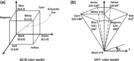
RGB is a fundamental way of representing color signal which is originated from cathode ray tube (CRT) display. The RGB model (Fig. 3) is represented by a 3-dimensional cube with R, G, and B at the corners on each axis. RGB is most dominantly used representation for processing and storing of digital image data. Therefore, it has been used in many skin color detection researches [36, 51, 61]. However, its poor separability between luminance and chromaticity information, and its highly sensitive nature against illumination variation are main limitations for skin color analysis purpose. Rather than original RGB format, its normalized variant is considered to be more robust in skin color detection since it reduces the dependency of each component to illumination changes² [38]. Normalized RGB representation can be obtained by normalizing RGB values by their intensity ( $$I=R+G+B$$

$\begin{aligned} r = \frac{R}{R+G+B}, \ g = \frac{G}{R+G+B}, \ b = \frac{B}{R+G+B} \end{aligned}$

(1)

where each RGB primaries are given in linear RGB³. Because $$r+g+b=1$$

, no information is lost if only two elements are considered.

Fig. 3

RGB cube and HSV hexcone representations

3.1.2 YCbCr

YCbCr is the Rec. 601 international standard (see 2) for studio quality component digital video. In YCbCr, color is represented by luma(Y), computed as a weighted sum of nonlinear (gamma-corrected) RGB ,and two chroma components Cr and Cb that are formed by subtracting luma value from R and B components. The Rec. 601 specifies 8 bit (i.e. 0–255) coding of YCbCr. All three Y, Cb, and Cr components have reserved ranges to provide footroom and headroom for signal processing as follows:

$\begin{aligned} {\left\{ \begin{array}{ll} Y' &{}= 16 + (65.738R' + 129.057G' + 25.064B') \\ Cb &{}= 128 + (-37.945R' - 74.494G' + 112.439B') \\ Cr &{}= 128 + (112.439R' - 94.154G' -18.285B') \\ \end{array}\right. } \end{aligned}$

(2)

where $R',G',B' \in [0,1]$ are gamma-corrected RGB primaries. YCbCr is dominantly used in compression applications since it reduces the redundancy in RGB color signals and represents the color with statistically independent components. The explicit separation of luminance and chrominance components and its wide adoption in image/video compression standards makes YCbCr popular for skin color analysis [7, 29, 33, 62].

3.1.3 HSV

The HSV coordinate system, originally proposed by Smith [57], defines color by: (i) Hue(H)—the property of a color related to the dominant wavelength in a mixed light wave, (ii) Saturation(S)—the amount of white light mixed with color that varies from gray through pastel to saturated colors, (iii) Value(V)—the property according to which an area appears to exhibit more or less light that varies from black to white. The HSV representation corresponds more closely to the human perception of color than aforementioned ones since it is derived from the intuitive appeal of the artist’s tint, shade, and tone. The set of equations used to transform a point in the RGB to the HSV coordinate system ( $[H,S,V] \in [0,1]$ , $[R',G',B'] \in [0,1]$ ) is given as follows⁴:

$\begin{aligned} {\left\{ \begin{array}{ll} H &{}= \frac{1}{6} \times {\left\{ \begin{array}{ll} 5+(M-B')/C \mathrm ,if M = R', m = G' \\ 1-(M-G')/C \mathrm ,if M = R', m \ne G' \\ 1+(M-R')/C \mathrm ,if M = G', m = B' \\ 3-(M-B')/C \mathrm ,if M = G', m \ne B' \\ 3+(M-G')/C \mathrm ,if M = B', m = R' \\ 5-(M-R')/C \mathrm ,if M = B', m \ne R' \end{array}\right. } \\ S &{}= C / M \quad \mathrm (if C=0, then H = undefined) \\ V &{}= M \end{array}\right. } , {\left\{ \begin{array}{ll} M= \max (R',G',B') \\ m= \min (R',G',B') \\ C= M-m \end{array}\right. } \end{aligned}$

(3)

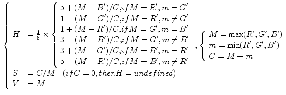
The HSV colorspace is traditionally shown as a hexcone model Fig. 3b and, in fact, HSV hexcone is a projection of the RGB cube along the gray-scale line. In hexcone model, H is represented as the angle and S corresponds to the horizontal distance from the vertical axis. V varies along the vertical axis with $$V=0$$

being black, and $$V=1$$

being white. When $$S=0$$

, color is a gray value. When $$S=1$$

, color is on the boundary of hexcone. The greater the S, the farther the color is from white/gray/black. Adjusting the hue varies the color from red at $$H=0$$

, through green at $$H=1/3$$

, blue at

, and back to red at $$H=0$$

. When

, or

, (along the achromatic axis) the color is grayscale and H is undefined.

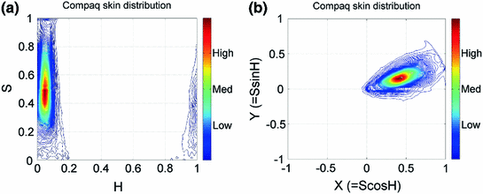
Two chromatic components, H and S, are known to be less variant to changes of illumination direction and illumination intensity [20], and thus HSV is a reliable colorspace for skin color detection. However, one should be careful in exploiting HSV space for skin color analysis since manipulation of H involves circular statistics as H is an angular measure [27]. As can be seen in Fig. 4a, the cyclic nature of H component disallows use of a color distribution model which requires a compact cluster, e.g. a single Gaussian model, since it generates two separate clusters on both sides of H axis. To address this issue, polar coordinate system of H-S space can be represented in Cartesian coordinates X-Y as follows [4]:

$\begin{aligned} X = S\cos (2\pi H), \quad Y = S\sin (2\pi H) \end{aligned}$

(4)

where $H,S \in [0,1]$ and $X,Y \in [-1,1]$ . Here, X component can be regarded as a horizontal projection of color vector representing a pixel in H-S space, while Y component can be regarded as a vertical projection of color vector representing a pixel in H-S space. In the Cartesian representation of H-S space (Fig. 4b), skin color distribution forms a tightly distributed cluster.

Fig. 4

Distribution of skin color pixel from Compaq dataset [36] in a H-S plane of original HSV colorspace, b Cartesian representation of H-S plane

3.2 Skin Color Distribution Model

Skin color distribution model defines a decision rule to discriminate between skin and non-skin pixels in given colorspace. To detect skin color pixel, a multitude of solutions merge from two distinct categories (Fig. 5). The first type of methodologies use a static color classification rule and can be further divided into three sub-classes depending on the classifier type: (i) piecewise boundary model [7, 23, 30, 42], (ii) non-parametric skin distribution model [4, 36, 77], (iii) parametric skin distribution model [45, 73, 74]. However, static skin color classification methods are typically very sensitive to imaging conditions, e.g. skin color of same individual varies depending on the color temperature of light source (e.g. incandescent, fluorescent, and sunlight) as well as the characteristics of image acquisition devices (e.g. sensor spectral sensitivity and embedded white balancing algorithm). Therefore, it requires appropriate adaptation schemes to maintain stable performance in real-world environments. The dynamic approaches address such problematic cases either by pre-processing given input image to alleviate the influence of imaging condition on color description or by dynamically updating color classification model according to imaging condition.

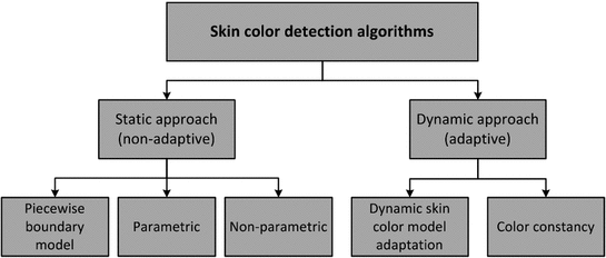
Fig. 5

Classification of skin color detection approaches

Since skin color typically forms a small cluster in the colorspace, one of the easiest methods to build a skin color classifier is to explicitly define fixed decision boundaries of skin regions. Single or multiple ranges of threshold values for each color component are defined and the image pixel values that fall within these pre-defined ranges are defined as skin pixels. Piecewise boundary model has been exploited in various colorspaces and Table 1 presents some representative examples.

Table 1

Commonly used piecewise boundary models for skin color detection

Authors (Colorspace)	Skin color classification rule
Kovac et al. [42] (RGB)	Uniform daylight illumination
	220, G>210, B>170, \|R-G\|\le 15, B
Gomez&Morales [23] (nRGB)	$$$\frac{r}{g}>1.185, \quad \frac{rb}{(r+g+b)^2} > 0.107, \quad \frac{rg}{(r+g+b)^2} > 0.112$$” src=”/wp-content/uploads/2016/03/A308467_1_En_12_Chapter_IEq26.gif”></SPAN> <SPAN id=IEq27 class=InlineEquation><IMG alt=$$^b$$ src=$
Chai&Ngan [7] (CbCr)	$77\le Cb\le 127, 133\le Cr\le 173$
Herodotou et al. [30] (HSV)	$0.94\le H\le 1 \mathrm or 0\le H\le 0.14, 0.2\le S, 0.35\le V ^d$

Non-parametric skin color modeling methods estimate the probability of a color value to be a skin by defining a model that has no dependency on a parameter. The most representative methods in this class is Jones and Rehg’s method [36] which uses a 2D or 3D color histogram to represent the distribution of skin color in colorspace. Under this approach, the given colorspace is quantized into a number of histogram bins and each histogram bin stores the likelihood that a given color belongs to the skin. Jones and Rehg built two 3D RGB histogram models for skin and non-skin from Compaq database [36] which contains around 12K web images. Given skin and non-skin histograms, the probability that a given color belongs to skin and non-skin class is defined as:

$\begin{aligned} p(\varvec{c}|w_s) = \frac{s(\varvec{c})}{\text {Total skin pixel count}} \quad , \quad p(\varvec{c}|w_n) = \frac{n(\varvec{c})}{\text {Total non-skin pixel count}} \end{aligned}$

(5)

where $s(\varvec{c})$ is the pixel count in the color bin $\varvec{c}$ of the skin histogram, $n(\varvec{c})$ is the pixel count in the color bin $\varvec{c}$ of the non-skin histogram. For skin pixel detection, we need to estimate $p(w_s|\varvec{c})$ —a probability of observing skin pixel given a $\varvec{c}$ color vector. To compute this probability, the Bayesian rule is applied using the given conditional probabilities of skin and non-skin:

$\begin{aligned} p(w_s|\varvec{c}) = \frac{p(\varvec{c}|w_s)p(w_s)}{p(\varvec{c}|w_s)p(w_s) + p(\varvec{c}|w_n)p(w_n)} \end{aligned}$

(6)

Instead of calculating the exact value of $p(w_s|\varvec{c})$ , the ratio between $p(w_s|\varvec{c})$ and $p(w_n|\varvec{c})$ can be compared (i.e. likelihood ratio test) for classification as follows:

$$$\begin{aligned} \varvec{c} \in w_s \mathrm ,if&\frac{p(w_s|\varvec{c})}{p(w_n|\varvec{c})} > K \nonumber \\ \Rightarrow \mathrm if&\frac{p(w_s|\varvec{c})}{p(w_n|\varvec{c})} = \frac{p(\varvec{c}|w_s)p(w_s)}{p(\varvec{c}|w_n)p(w_n)} > K \\ \Rightarrow \mathrm if&\frac{p(\varvec{c}|w_s)}{p(\varvec{c}|w_n)} > \theta \mathrm ,where \theta = K \times \frac{p(w_n)}{p(w_s)}\nonumber \end{aligned}$$” src=”/wp-content/uploads/2016/03/A308467_1_En_12_Chapter_Equ7.gif”></DIV></DIV><br /> <DIV class=EquationNumber>(7)</DIV></DIV>where <SPAN id=IEq40 class=InlineEquation><IMG alt=$ is an adjustable threshold that controls the trade-off between true positive (TP) and false positive (FP) rates (See 13 for definitions of TP and FP).

The third categories in static approaches are parametric skin color modeling methods where color classification rule is derived from parameterized distributions. The parametric models have the advantage over the non-parametric ones that they require smaller amount of training data and storage space. Key problems for parametric skin color modeling are to find the best model and to estimate its parameters. The most popular solutions include single Gaussian model (SGM) [73], Gaussian mixture model (GMM) [24, 32, 74], and elliptical model [45].

Under controlled environment, skin colors of different subject cluster in a small region in the colorspace and hence, the distribution can be represented by SGM [73]. A multivariate Gaussian distribution of a $$d$$

-dimensional color vector $\varvec{c}$ is defined as:

$\begin{aligned} G(\varvec{c};\varvec{\mu }, \Sigma ) = \frac{1}{(2 \pi )^{d/2} |\Sigma |^{1/2}} \exp \left[ -\frac{(\varvec{c}-\varvec{\mu })^T \Sigma ^ {-1} (\varvec{c}-\varvec{\mu })}{2} \right] \end{aligned}$

(8)

where $\varvec{\mu }$ is the mean vector and $\Sigma$ is the covariance matrix of the normally distributed color vector $\varvec{c}$ . The model parameters are estimated from the training data using the following equations:

$\begin{aligned} \varvec{\mu } = \frac{1}{n} \sum ^n_{i=1} \varvec{c}_i , \Sigma = \frac{1}{n-1} \sum ^n_{i=1} (\varvec{c}_i-\varvec{\mu })(\varvec{c}_i-\varvec{\mu })^T \end{aligned}$

(9)

Either the $G(\varvec{c};\varvec{\mu }, \Sigma )$ probability or the Mahalanobis distance from the $\varvec{c}$ color vector to the mean vector $\varvec{\mu }$ , given the covariance matrix $\Sigma$ , can be used to measure the similarity of the pixel with the skin color.

Although SGM has been a successful model to represent skin color distribution, the assumption of SGM requires a single cluster which smoothly varies around the mean. However, such an assumption often causes intolerable error in skin/non-skin discrimination since different modes (due to skin color types and varying illumination conditions) can co-exist within the skin cluster. Therefore, Yang and Ahuja introduced the GMM model [74] to represent more complex shaped distribution. The GMM probability density function (pdf) can be defined as a weighted sum of Gaussians:

$\begin{aligned} p(\varvec{c};\alpha _i,\varvec{\mu }_i, \Sigma _i) = \sum _{i=1}^N \alpha _i G_i(\varvec{c};\varvec{\mu }_i,\Sigma _i) \end{aligned}$

(10)

where

is the number of mixture components, $\alpha _i$ is the weight of i-th component ( $$$\alpha _i > 0$$” src=”/wp-content/uploads/2016/03/A308467_1_En_12_Chapter_IEq52.gif”></SPAN>, <SPAN id=IEq53 class=InlineEquation><IMG alt=$ ), $$G_i$$

is a Gaussian pdf with parameters $\varvec{\mu }_i$ and $\Sigma _i$ . The parameters of a GMM are approximated from the training data via the iterative expectation-maximization (EM) technique [11].

Lee and Yoo [45] claimed that SGM is not accurate enough to approximate the skin color distribution because of the asymmetry of the skin cluster with respect to its density peak. They proposed an elliptical boundary model based on their observations that the skin cluster is approximately elliptic in shape. The elliptical boundary model is defined as:

$\begin{aligned} \Phi (\varvec{c}) = (\varvec{c}-\varvec{\phi })^T \Lambda ^{-1}(\varvec{c}-\varvec{\phi }) \end{aligned}$

(11)

$\varvec{\phi }$ and $\Lambda$ are two model parameters to be estimated from training data:

$\begin{aligned} \varvec{\phi } = \frac{1}{n} \sum _{i=1}^n \varvec{c}_i \quad , \quad \Lambda = \frac{1}{N} \sum _{i=1}^n f_i(\varvec{c}_i-\varvec{\mu })(\varvec{c}_i-\varvec{\mu })^T \quad , \quad \varvec{\mu } = \frac{1}{N} \sum _{i=1}^n n f_i \varvec{c}_i \end{aligned}$

(12)

where

is the number of distinctive training color vectors $\varvec{c}_i$ of the training skin pixels, $$f_i$$

is the number of skin samples of color vector $\varvec{c}_i$ , and $$N$$

is the total number of samples ( $N = \sum _{i=1}^n n f_i$ ). An input pixel $\varvec{c}$ is classified as skin if $\Phi (\varvec{c})<\theta$ where $\theta$ is a threshold value.

3.3 Comparison and Discussion of Skin Color Distribution Models and Color Representations

Comparative assessment of skin color detection methods in different color representations has been discussed in many literatures [8, 41, 51, 53, 60, 63, 64], but they report different results mainly due to their different experimental conditions (e.g. selection of training/testing datasets). In this section, we will highlight some general conclusions derived from existing researches. Typically, the performance of skin color detection is measured using true positive rate (TPR) and false positive rate (FPR), defined as follows:

$\begin{aligned} TP =&\frac{\text {number of correctly identified skin pixels}}{\text {total number of skin pixels}} \nonumber \\ FP =&\frac{\text {number of falsely identified non-skin pixels as skin pixels}}{\text {total number of non-skin pixels}} \end{aligned}$

(13)

Most classification methods have an adjustable threshold parameter that controls the classifier decision boundary. As a result, each threshold value produces a pair of FP and TP values, generating a receiver operating characteristics (ROC) curve which demonstrates the relationship between TP and FP in different threshold values. For comparative evaluation of different classifiers, ROC performance is often summarized by a single scalar value, the area under ROC curve (AUC). AUC is known to be a fairly reliable performance measure of the classifier [14]. Since the AUC is a subregion of the unit square, its value lies between 0 and 1, and larger AUC value implies better classification performance.

A piecewise boundary model has fixed decision boundary parameters and hence, the corresponding ROC plots have only one point. Its boundary parameter values differ from one colorspace to another and one illumination to another. Although methods in this category are computationally fast, in general, they suffer from high FP rates. For example, Phung et al. [51] indicated that piecewise boundary classifier in CbCr space [7] achieves $92\,\%$ TP at $28\,$ FP on Edith Cowan University (ECU) dataset [51] (consists of 4K color images from web or taken with digital camera, containing skin pixels), while both 3D SGM classifier of skin/non-skin (YCbCr) and Bayesian classifier with 3D histogram (RGB) achieves higher than $95\,\%$ TP at the same FP.

The Gaussian distribution based classifiers, e.g. SGM and GMM, and an elliptical model classifier have been widely used for skin color analysis since they generalize well with small amount of training data. In order to compare the performance of SGM and GMM, Caetano et al. [6] conducted comparative evaluation in normalized-rg colorspace using a dataset of 800 images from various ethnic groups (publicly not available). The authors noted that: i) GMM generally outperforms SGM for FP rates higher than $10\,\%$ , while both models yield similar performance for low FP rates, ii) detection performance remains unchanged except minor fluctuations when increasing mixture components for GMM from 2 to 8. Fu et al. [18] performed similar comparative assessment of both Gaussian classifiers using Compaq dataset [36] and confirmed that increasing mixture components doesn’t provide significant performance improvement for

$$n>5$$” src=”/wp-content/uploads/2016/03/A308467_1_En_12_Chapter_IEq72.gif”></SPAN> in four representative colorspaces (RGB, YCbCr, HSV, and normalized RGB). This is due to an overfitting issue, implying that a classifier describes training sample well but is not flexible enough to describe general samples. Moreover, using GMM is slower during classification since multiple Gaussian components must be computed to obtain the probability of a single color value. Therefore, one should be careful in selecting appropriate number of mixture components.</DIV><br />
<DIV class=Para>The performance of the representative non-parametric method, Bayesian classifier with 3D histogram [<CITE><A href=

36], has been compared with other parametric approaches in [36, 51]. The histogram technique in 3D RGB color space achieved $90\,\%$ TP ( $14.2\,$ FP) on Compaq database, slightly outperforming GMM or SGM in terms of detection accuracy. But it requires a very large training dataset to get a good classification rate, as well as higher storage space. For example, a 3D RGB histogram with 256 bins per channel requires more than 16 millions entries. To address this issue, some literature presented color bin quantization method to reduce color cube size. Jones and Rehg [36] compared the use of different numbers of histogram bins $$(256^3,32^3,16^3)$$

and found that $$32^3$$

histogram performed best, particularly when small amount of training data was used.

Often, skin detection methods solely based on color cue in Sect. 3.2 (summarized in Table 2) are not sufficient for distinguishing between skin regions and skin-colored background regions. In order to minimize false acceptance of skin-colored background objects as skin regions, textural and spatial properties of skin pixels can be exploited [10, 40, 69]. Such methods generally rely on the facts that skin texture is smoother than other skin similar areas. For example, Wang et al. [69] initially generated a skin map via pixel-wise color analysis, then carried out texture analysis using Gray-Level Co-occurrence Matrices (GLCM) features to refine the original skin map (i.e. remove false positives). Khan et al. [40] proposed a systematic approach employing spatial context in conjunction with color cue for robust skin pixel detection. At first, a foreground histogram of probable skin colors and a background histogram of the non-skin colors are generated using skin pixel samples in the input image extracted via a face detector. These histograms are used to compute foreground/background weights per pixel, representing the probability of each pixel being skin or non-skin. Subsequently, spatial context is taken into account by applying the graph-cut based segmentation on basis of computed weights, producing segmented skin regions of reduced false positives.

Table 2

Summary of various skin color detection methods (In characteristic column, $$+$$

and

represents pros and cons respectively)

Category	Method	Characteristic
Piecewise boundary	Chai (YCbCr) [7], Gomez (normalized RGB) [23], Herodotou (HSV) [30], Kovac (RGB) [42]	Simple implementation Limited flexibility due to fixed threshold and high false positive rate
Non-parametric	Brown’s self organizing map (SOM) [4], Jones’s Bayesian approach with 3D histogram [36], Zarit’s lookup table (LUT) [77]	Higher detection accuracy and less dependency on choice of colorspace Require larger amount of training data and storage compared to parametric solutions
Parametric	Single Gaussian Model [73], Gaussian Mixture Model [24, 32, 74], Lee’s elliptical model [45]	Better generalization with less training data Potential long training delay (for mixture model) and high dependency on choice of colorspace

Selection of the best colorspace for skin classification is a very challenging task. This problem has been analyzed in numerous literatures with various combinations of skin color distribution models and training/testing datasets. In general, effectiveness of specific color representation in skin color detection can be measured based on their separability between skin and non-skin pixels, and robustness towards illumination variation. However, there is no single best colorspace that is clearly superior to others in all images and often only marginal improvement can be achieved by choice of colorspace.

The effectiveness of colorspace is also dependent on selection of skin color distribution model. For example, non-parametric models, such as histogram-based Bayes classifier are less sensitive to colorspace selection compared to parametric modeling schemes, such as SGM and GMM [1, 38, 65]. Some literatures indicate that transforming 3D colorspace to 2D by discarding the luminance component may enhance skin detection performance since chrominance components are more important cue for determination of skin color. However, elimination of luminance component should be avoided since it decreases classification performance [1, 38, 53], and therefore, is not recommended unless one wants to have faster solution (due to dimensionality reduction) at the cost of classification accuracy.

3.4 Illumination Adaptation for Skin Color Detection

Most of the skin color detection methodologies presented in Sect. 3.2 remain stable only to slight variation in illumination since the appearance of color is heavily dependent on the illumination condition under which the object is viewed. In order to maintain reliable performance over a wide range of illumination conditions, several illumination adaptation schemes have been proposed, which can be subdivided into two main approaches [38]: (i) Dynamic model adaptation: by updating trained skin color models dynamically according to the illumination and imaging conditions, (ii) Color constancy: by pre-processing an input image to produce a transformed version of the input as if the scene is rendered under standard illumination condition.

3.4.1 Dynamic Adaptation of Skin Color Model

Dynamic model adaptation approaches usually depend on the results of high-level vision tasks such as face detection and tracking to improve skin color detection performance. Sigal et al. [55

Only gold members can continue reading. Log In or Register to continue