Fig. 1
Example of reference Data. Each vertebra is assigned a unique label (color coded). Left Sagittal view, right 3D view
4 Participating Algorithms
There are over 60 requests or downloads of the training data from SpineWeb. Five teams entered the challenge held at the Computational Spine Imaging workshop (CSI2014). Among the participants, four teams segmented both thoracic and lumbar spines, and one team only segmented the lumbar spine.
The five participating algorithms are dubbed as Method 1 [11], Method 2 [12], Method 3 [13], Method 4 [14], and Method 5 [15] in this paper according to the order of the submission. The titles of the five methods are listed in the bibliography. The technical comparisons of the five methods are conducted in six aspects: localization, model, bundled model, registration/optimization, feature function and running time. Method 1 and Method 4 comprise steps to automatically localize and initialize the vertebrae. Method 2, 3, and 5 require manual initialization of the model, either at the center of the vertebral body or at the endplates. All methods are based on certain type of shape and intensity models. Method 1 uses multiple atlases directly derived from the reference data. Method 2 uses statistical shape  pose model built from 87 training models. Both Method 3 and Method 4 use mean shape models. Method 4 builds a model for each vertebra level, while Method 3 builds one model for each spine section (one for T1–T6, one for T7–T12, and one for L1–L5). Method 5 computes a statistical shape model from 30 training models for each vertebra level. In Method 1 and Method 2, adjacent vertebrae are bundled together (5 vertebrae in Method 1 and 3 vertebrae in Method 2) in the segmentation. Different registration/optimization frameworks were adopted in the methods. Method 1 first applies a non-rigid registration for each atlas and then performs a label fusion. Method 2 conducts an EM algorithm to optimize the model. Method 3 adopts a total variation framework. Surface mesh deformation and reconfiguration is performed in Method 4. Method 5 employs statistical shape deformation plus b-spline relaxation for the surface optimization. Different feature functions are used in the methods for the optimization. They are mostly based on edge point and intensity model. The running time was reported by the participating teams as follows. Method 1-5 takes approximately 12, 10, 60, 30 and 3 minutes per case respectively. It can only be viewed as a reference since the algorithms were run on different hardware and some have been optimized by GPU.
pose model built from 87 training models. Both Method 3 and Method 4 use mean shape models. Method 4 builds a model for each vertebra level, while Method 3 builds one model for each spine section (one for T1–T6, one for T7–T12, and one for L1–L5). Method 5 computes a statistical shape model from 30 training models for each vertebra level. In Method 1 and Method 2, adjacent vertebrae are bundled together (5 vertebrae in Method 1 and 3 vertebrae in Method 2) in the segmentation. Different registration/optimization frameworks were adopted in the methods. Method 1 first applies a non-rigid registration for each atlas and then performs a label fusion. Method 2 conducts an EM algorithm to optimize the model. Method 3 adopts a total variation framework. Surface mesh deformation and reconfiguration is performed in Method 4. Method 5 employs statistical shape deformation plus b-spline relaxation for the surface optimization. Different feature functions are used in the methods for the optimization. They are mostly based on edge point and intensity model. The running time was reported by the participating teams as follows. Method 1-5 takes approximately 12, 10, 60, 30 and 3 minutes per case respectively. It can only be viewed as a reference since the algorithms were run on different hardware and some have been optimized by GPU.5 Evaluation
The performance on the training set was evaluated by participants and reported in their submissions to the workshop. The performance of the test set was evaluated by the challenge organizers.
After the test data was released in July, the participants were given 10 days to submit the segmentation results. Each segmented vertebra was assigned a unique label. The results were submitted in Meta format (MHD/raw) with the same resolution of the original CT data.
Two metrics were employed for evaluation: dice coefficient (DC) and absolute surface distance (ASD). The evaluation was conducted on each individual vertebra.
By visual inspection, we notice that the segmentation performed differently at different parts of the vertebra. Therefore we evaluate the segmentation performance for both the whole vertebra and its four substructures: vertebra body, left transverse process, right transverse process, and spinal process. We developed an automatic method to partition the vertebra into anatomical substructures [16]. It is based on the anatomical knowledge that pedicles and laminae are the densest parts of the vertebral arch which forms the circle of bones around the spinal canal. We therefore search for the four cutting planes at left pedicle, right pedicle, left lamina and right lamina that go through the cross-sections with highest CT intensity around the spinal canal. Symmetric constraints are also enforced to balance the left and right cutting planes. The vertebra is then partitioned into four substructures (vertebral body, left transverse process, right transverse process and spinal process depending on which side of the cutting planes a pixel lies. Figure 2 shows the partitioning of a vertebra into four substructures.

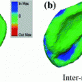
Fig. 2
Partitioning of a vertebra into four substructures. Left Density map on vertebra surface, hotter color: higher density. Right Partitioning a vertebra into four substructures. The substructures are color-coded with different colors. The cutting planes lie at the border between two substructures
6 Performance Comparison
The segmentation results were compared both visually and quantitatively. The segmentation result was superimposed on the CT image for visual inspection. Dice coefficient (DC) and absolute surface distance (ASD) were used for quantitative analysis. In this paper, we mainly focus on the results on the test set.


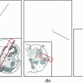
Fig. 3
Visual comparison of segmentation results for test case
Fig. 4
Visual comparison of segmentation results for specific vertebrae in test case 5. Row 1 T3 vertebra; Row 2 T9 vertebra; Row 3 L3 vertebra Mid-axial slice for each vertebra is shown. The segmentation is superimposed on the CT data
Figure 3 shows the visual comparison of submitted segmentation results for test case 1. All methods achieve visually acceptable segmentation for the thoracolumbar spine column. There is no overly leakage or under-segmentation from the sagittal view. For a closer visual inspection, Fig. 4 shows the visual comparison of the segmentation of the mid-axial slice for three representative vertebrae: T3, T9 and L3. In T3 and T9, all methods successfully separate the vertebra and the ribs. The border of segmented vertebra in Method 1is not smooth, which indicates further refinement is necessary. The segmentation in Method 2 is off-mark although the location of the vertebra and the overall shape are correct. Another stage of local segmentation should be conducted. Method 3 and 4 both get pretty good segmentation results, but it is noted that the segmentation of the posterior substructures still have rooms for improvement. The tips of the processes are not completely segmented and some contrast-enhanced vessels are included in the segmentation. Method 5 only segments the lumbar spine and the result is similar to that of Method 1 where the boundary is slightly off.
Figure 5 shows the average dice coefficient for all five methods from T1 to L5. There is a general trend of better performance from upper spine to lower spine as the vertebrae gradually increase the size and density. Both DC and ASD show the same pattern. To further illustrate the pattern, we group the vertebrae into three sections: upper thoracic from T1 to T6, lower thoracic from T7 to T12 and lumbar spine from L1 to L5. The DC goes from 0.867 in the upper thoracic, to 0.909 in the lower thoracic and to 0.933 in the lumbar spine.

Fig. 5
Mean performance of all methods at each vertebra level
Related posts:
 Models for Descriptive Patient-Specific Neuro-Anatomical Modeling: Towards a Digital Brainstem Atlas
 Supervised Segmentation and Meshing of 3D Intervertebral Discs of the Lumbar Spine for Discectomy Simulation
 Active Optical Flow Model for Dose Prediction in Spinal SBRT Plans
 Auto-encoders for Classification of 3D Spine Models in Adolescent Idiopathic Scoliosis
Stay updated, free articles. Join our Telegram channel

Full access? Get Clinical Tree


