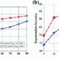
and Dice coefficient of  indicate that accurate segmentation can be obtained by the described framework. Moreover, when compared to the complete graph, the computational time was reduced by a factor of approximately nine in the case of optimal assignment-based shape representation.
1 Introduction
Segmentation of vertebrae is among the most challenging segmentation problems, as vertebrae are highly articulated structures, consisting of the vertebral body, pedicles and processes. As a result, the application of unsupervised segmentation approaches is limited, however, supervised segmentation approaches that require prior modeling of vertebral structures were already successfully applied, especially in the case of three-dimensional (3D) spine images [1–7]. For the segmentation of vertebral and also other anatomical structures, shape modeling has been mostly driven by active shape models (ASM) [8] and active appearance models (AAM) [9]. However, if the distance between the initial model and the object of interest is too large, model optimization may lead to an incorrect solution that is locally but not globally optimal. Moreover, intensities and shapes are generally treated separately and independently. To overcome these shortcomings, landmark-based segmentation methods, where the object of interest is described by intensity and shape properties of landmarks and connections among these landmarks, have been proposed [10–12]. However, methods that were originally developed for two-dimensional (2D) images cannot be directly applied to 3D images, because a considerably larger number of landmarks is required to accurately capture the shape of the object of interest in 3D. If the number of landmarks increases linearly, the number of connections among landmarks exhibits a quadratic growth, which is reflected in the computational complexity. In the case the shape is represented by a complete set of connections among landmarks (i.e. a complete graph), the resulting shape representation is strong and prevents non-plausible shape deformations in 2D, but may at the same time limit the shape elasticity in 3D. A balance among computational complexity, rigidity and elasticity may be obtained by reducing the complete set of connections [13], and the more recent approaches combined statistical properties of individual connections, defining local shape properties, and of the complete set of connections, defining global shape properties [11, 14]. Despite considerable improvements, existing approaches often result in a discriminative degree of connections for different landmarks, i.e. the number of connections established for different landmarks varies. In practice, this usually reflects in a high degree of connections for few landmarks and a low degree for most landmarks, which may lead to errors in landmark detection and formation of non-plausible shapes.
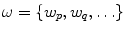
In this paper, we combine a non-discriminative landmark-based shape representation [15] with a landmark-based segmentation framework [12] and extend its application from 2D to 3D image segmentation (Fig. 1). The introduced 3D shape representation is based on concepts from transportation theory [16], and is integrated with a landmark-based detection in 3D that relies on concepts from game theory [17]. The resulting framework was validated for segmentation of lumbar vertebrae from 3D computed tomography (CT) spine images.
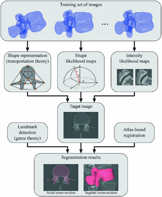
Fig. 1
An overview of the proposed segmentation framework. The 3D shape representation of the object of interest is determined by connections among landmarks that are established according to the optimal assignment, a special case of transportation theory. The shape and intensity likelihood maps are also computed for landmarks in images from the training set, and together with the shape representation used to guide landmark detection in the target image, which is based on concepts from game theory. The resulting landmarks in the target image are combined with an atlas-based image registration that combines landmarks and pre-segmented surfaces of the object of interest in the training set of images with landmarks in the target image to generate the final segmentation results in 3D
2 Methodology
2.1 Transportation Theory
Transportation theory [16], originally developed in the field of applied economy, is focused on solving problems related to transporting goods and allocating resources between sources and destinations, and provides globally optimal solutions for a variety of applications based on graph theory. In the field of image analysis, transportation theory has already been applied to solve various problems related to information matching and comparison. In this paper, we apply transportation theory to determine the optimal landmark-based shape representation of the object of interest. In the case the object of interest is described by landmarks  , its landmark-based shape representation can be defined by connections among pairs of landmarks
  ;
;  . The most straightforward approach is to establish connections for every pair of landmarks, which results in the complete graph of
 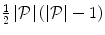 connections, where
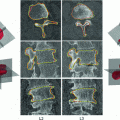
  is the number of landmarks. As the complete graph-based shape representation is relatively rigid, its application in segmentation will in general not result in non-plausible shapes, but some shapes that are plausible may not be detected due to its limited elasticity. Because a connection is established for every pair of landmarks, the resulting shape representation is also relatively complex. Although these limitations may not be of utmost importance in the case of 2D shapes, they may be emphasized in the case of 3D shapes, where the number of landmarks and corresponding connections can be considerably larger. To balance the rigidity, elasticity and complexity of the shape representation, connections among landmarks can be selectively established by various approaches [13]. However, existing approaches may result in unequal degrees of connections among landmarks (Fig. 2a), which may lead to non-plausible shapes. We therefore propose a novel non-discriminative statistical shape representation, where we selectively establish connections and, at the same time, enforce equal degrees of connections among landmarks. The process of establishing optimal connections is guided by statistical properties of landmarks, learned from the training set of images and then applied to the target image, and is observed from the perspective of transportation theory. For our purpose, we exploit a special case of allocating sources to destinations in a one-to-one manner called the optimal assignment, because it has several computationally effective solutions, e.g. the Hungarian algorithm [18].
, its landmark-based shape representation can be defined by connections among pairs of landmarks ; . The most straightforward approach is to establish connections for every pair of landmarks, which results in the complete graph of connections, where is the number of landmarks. As the complete graph-based shape representation is relatively rigid, its application in segmentation will in general not result in non-plausible shapes, but some shapes that are plausible may not be detected due to its limited elasticity. Because a connection is established for every pair of landmarks, the resulting shape representation is also relatively complex. Although these limitations may not be of utmost importance in the case of 2D shapes, they may be emphasized in the case of 3D shapes, where the number of landmarks and corresponding connections can be considerably larger. To balance the rigidity, elasticity and complexity of the shape representation, connections among landmarks can be selectively established by various approaches [13]. However, existing approaches may result in unequal degrees of connections among landmarks (Fig. 2a), which may lead to non-plausible shapes. We therefore propose a novel non-discriminative statistical shape representation, where we selectively establish connections and, at the same time, enforce equal degrees of connections among landmarks. The process of establishing optimal connections is guided by statistical properties of landmarks, learned from the training set of images and then applied to the target image, and is observed from the perspective of transportation theory. For our purpose, we exploit a special case of allocating sources to destinations in a one-to-one manner called the optimal assignment, because it has several computationally effective solutions, e.g. the Hungarian algorithm [18].Fig. 2
a A shape representation consisting of 13 landmarks with unequal degrees of connections. b Separation of landmarks into two clusters of 6 and 7 landmarks (note that the cardinality of clusters is equalized by a pseudo-landmark). Intra-cluster connections are established as complete graphs. c Optimal assignment-based shape representation, consisting of intra-cluster and also inter-cluster connections (in green), established by optimal assignment among landmarks in the two clusters
2.2 Game Theory
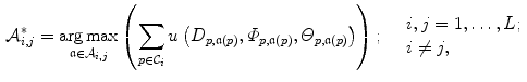
Game theory [17] is a discipline that studies the behavior of decision makers, who play a game by making decisions that impact one another. A game is a set of rules for playing, and a play is a specific combination of these rules that occurs when each player (i.e. the decision maker) chooses a strategy (i.e. a decision as an admissible behavior of the decision maker) so that it maximizes his payoff (i.e. the benefit gained according to the behavior of other players). In non-cooperative games, each player acts independently and aims to maximize his payoff regardless of payoffs gained by other players, while in cooperative games, players can join into coalitions (the grand coalition joins all players) and aim to maximize their joint payoff. In this paper, we apply game theory to detect the optimal position of landmarks that describe the object of interest. Landmark detection is considered as a game where landmarks are players, landmark candidate points are strategies, and likelihoods that each candidate point represents a landmark are payoffs [12]. As players (i.e. landmarks) can simultaneously participate in maximizing their joint payoffs (i.e. cumulative likelihoods) through the corresponding strategies (i.e. landmark candidate points), landmark detection in the target image can be represented as a cooperative game with the grand coalition and solved by maximizing the joint payoff  :
:
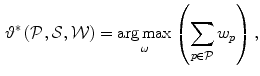
where  and
and 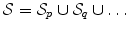 are, respectively, sets of landmarks and landmark candidate points,
  is the payoff for landmark
  ,
,  is an admissible combination of payoffs, and
  is the payoff matrix that consists of matrices
  of partial payoffs for each pair of landmarks
  . The element of
  at location
  represents the partial payoff of landmark
  if landmarks
  and
and  are represented by, respectively, candidate points
  and
and  .
.
:(1)
and are, respectively, sets of landmarks and landmark candidate points, is the payoff for landmark , is an admissible combination of payoffs, and is the payoff matrix that consists of matrices of partial payoffs for each pair of landmarks . The element of at location represents the partial payoff of landmark if landmarks and are represented by, respectively, candidate points and .2.3 Optimal Assignment-Based 3D Shape Representation
Let the object of interest be in each image from the training set  annotated by corresponding landmarks
  . The application of optimal assignment to all landmarks would result in a weak shape representation, because every landmark would be connected to only one other landmark (i.e. the degree of connections would be equal to one). To avoid such situation, we first divide landmarks into
  clusters, each with the same number of landmarks
  , so that
  (if the same cardinality cannot be achieved for every cluster, it is equalized by introducing pseudo-landmarks). Landmarks within each
  th cluster are connected by a complete graph
  , resulting in intra-cluster connections (Fig. 2b). For all clusters, the total number of intra-cluster connections is therefore
  . Moreover, each landmark from
  th cluster is connected to exactly one landmark from every other
  th cluster, resulting in inter-cluster connections (Fig. 2c). For all clusters, the total number of inter-cluster connections is therefore
  . The inter-cluster connections are defined by the optimal assignment
  that corresponds to the maximal total benefit of a shape representation [18]:
where  is the set of all possible one-to-one assignments among landmarks between
  th and
  th cluster in the form of bijections
  ,
,  is the landmark from
  th cluster that is assigned to landmark
  from
from  th cluster by bijection
  , and
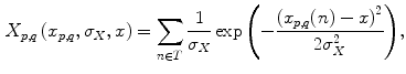
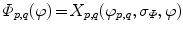
, and  is a linear function that is composed of probability distributions of distances
  , azimuth angles
  and polar angles
  . These probability distributions describe the 3D spatial relationships, observed in the spherical coordinate system, between any two landmarks
  that occur in images from the training set and are computed as:
where  is the feature value for landmarks
  and
and  in the
  th image from the training set
  ,
,  is an arbitrary feature value (
 ), and
  is a predefined constant that tunes the sensitivity of the distribution to feature value variations. The resulting distance, azimuth angle and polar angle distributions are therefore, respectively,
 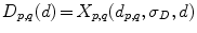 ,
,  and
and  , where
  is the distance,
  is the azimuth angle, and
  is the polar angle between landmarks
  and
and  .
.
annotated by corresponding landmarks . The application of optimal assignment to all landmarks would result in a weak shape representation, because every landmark would be connected to only one other landmark (i.e. the degree of connections would be equal to one). To avoid such situation, we first divide landmarks into clusters, each with the same number of landmarks , so that (if the same cardinality cannot be achieved for every cluster, it is equalized by introducing pseudo-landmarks). Landmarks within each th cluster are connected by a complete graph , resulting in intra-cluster connections (Fig. 2b). For all clusters, the total number of intra-cluster connections is therefore . Moreover, each landmark from th cluster is connected to exactly one landmark from every other th cluster, resulting in inter-cluster connections (Fig. 2c). For all clusters, the total number of inter-cluster connections is therefore . The inter-cluster connections are defined by the optimal assignment that corresponds to the maximal total benefit of a shape representation [18]:(2)
is the set of all possible one-to-one assignments among landmarks between th and th cluster in the form of bijections , is the landmark from th cluster that is assigned to landmark from th cluster by bijection , and is a linear function that is composed of probability distributions of distances , azimuth angles and polar angles . These probability distributions describe the 3D spatial relationships, observed in the spherical coordinate system, between any two landmarks that occur in images from the training set and are computed as:(3)
is the feature value for landmarks and in the th image from the training set , is an arbitrary feature value (), and is a predefined constant that tunes the sensitivity of the distribution to feature value variations. The resulting distance, azimuth angle and polar angle distributions are therefore, respectively, , and , where is the distance, is the azimuth angle, and is the polar angle between landmarks and .The resulting optimal assignment  between
  th and
  th cluster defines the set
 Monitoring of Syndesmophyte Growth in Ankylosing Spondylitis Using Computed Tomography
 Robust Segmentation Framework for Spine Trauma Diagnosis
 Detection and Labelling in Lumbar MR Images
 of Spinal Deformities Using a Parametric Torsion Estimator
 Based Tensor Level Set Framework for Vertebral Body Segmentation
 Segmentation and Discrimination of Connected Joint Bones from CT by Multi-atlas Registration


between th and th cluster defines the set
Related posts:
Robust Segmentation Framework for Spine Trauma Diagnosis
Based Tensor Level Set Framework for Vertebral Body Segmentation
Stay updated, free articles. Join our Telegram channel
Full access? Get Clinical Tree
