of a set of  landmarks
  on each, a statistical shape model is trained by applying principal component analysis (PCA) to the aligned shapes [2]. This yields a linear model of shape variation, which represents the position of each landmark
  using
using

(1)
 is the mean position of the point in a suitable reference frame,
  is a set of modes of variation,
  are the shape parameters,
  allows small deviations from the model, and
  applies a global transformation (e.g. similarity) with parameters
  .
.To match the model to a query image,  , the overall quality of fit
  , of the model to the image is optimised over parameters

where  is a cost image for the fitting of landmark
  ,
,  is the covariance matrix of shape model parameters
  ,
,  is a threshold on the Mahalanobis distance, and
  is a threshold on the residuals.
  is chosen using the cumulative distribution function (CDF) of the
  distribution so that 98 % of samples from a multivariate Gaussian of the appropriate dimension would fall within it. This ensures a plausible shape by assuming a flat distribution for model parameters
  constrained within hyper-ellipsoidal bounds [2]. In the original work [2],
  was provided by normalised correlation with a globally constrained patch model.
 , the overall quality of fit
  , of the model to the image is optimised over parameters

(2)
 is a cost image for the fitting of landmark
  ,
,  is the covariance matrix of shape model parameters
  ,
,  is a threshold on the Mahalanobis distance, and
  is a threshold on the residuals.
  is chosen using the cumulative distribution function (CDF) of the
  distribution so that 98 % of samples from a multivariate Gaussian of the appropriate dimension would fall within it. This ensures a plausible shape by assuming a flat distribution for model parameters
  constrained within hyper-ellipsoidal bounds [2]. In the original work [2],
  was provided by normalised correlation with a globally constrained patch model.
RF Regression Voting in the CLM Framework. In RFRV-CLM,  in Eq. 2 is provided by voting with a Random-Forest (RF) regressor. To train the RF for a single landmark, the shape model is used to assess the global pose,
  , of the object in each image by minimising
  . Each image is resampled into a standardised reference frame by applying the inverse of the estimated pose. The model is scaled so that the width of the reference frame of the mean shape is a given value,
  . Sample patches of area
  are then generated from the resampled images at a set of random displacements from the true point positions. The displacements
  are drawn from a flat distribution in the range
 ![$$[-d_{ max},+d_{ max}]$$](/wp-content/uploads/2016/10/A331518_1_En_14_Chapter_IEq30.gif) in
in  and
and  . Finally, image features
  are extracted from the sample patches. Haar-like features [20] are used, as they have proven effective for a range of applications and can be calculated efficiently from integral images. To allow for inaccurate initial estimates of the pose and to make the detector locally pose-invariant, the process is repeated with random perturbations in scale and orientation of the pose estimate. A RF [1] is then trained, using a standard, greedy approach, with the feature vectors
  as inputs and the displacements
  as regression targets. Each tree is trained on a bootstrap sample of
  pairs
pairs  from the training data. At each node, a random sub-set of
  features are chosen from this sample, and a feature
  and threshold
  that best split the data into two compact groups are selected by minimising an entropy measure [3]. Splitting terminates at either a maximum depth,
  , or a minimum number of samples,
  . The process is repeated to generate a forest of size
  .
.
 in Eq. 2 is provided by voting with a Random-Forest (RF) regressor. To train the RF for a single landmark, the shape model is used to assess the global pose,
  , of the object in each image by minimising
  . Each image is resampled into a standardised reference frame by applying the inverse of the estimated pose. The model is scaled so that the width of the reference frame of the mean shape is a given value,
  . Sample patches of area
  are then generated from the resampled images at a set of random displacements from the true point positions. The displacements
  are drawn from a flat distribution in the range
 ![$$[-d_{ max},+d_{ max}]$$](/wp-content/uploads/2016/10/A331518_1_En_14_Chapter_IEq30.gif) in
in  and
and  . Finally, image features
  are extracted from the sample patches. Haar-like features [20] are used, as they have proven effective for a range of applications and can be calculated efficiently from integral images. To allow for inaccurate initial estimates of the pose and to make the detector locally pose-invariant, the process is repeated with random perturbations in scale and orientation of the pose estimate. A RF [1] is then trained, using a standard, greedy approach, with the feature vectors
  as inputs and the displacements
  as regression targets. Each tree is trained on a bootstrap sample of
  pairs
pairs  from the training data. At each node, a random sub-set of
  features are chosen from this sample, and a feature
  and threshold
  that best split the data into two compact groups are selected by minimising an entropy measure [3]. Splitting terminates at either a maximum depth,
  , or a minimum number of samples,
  . The process is repeated to generate a forest of size
  .
.RFRV-CLM Fitting Fitting to a query image is initialised via an estimate of the pose of the model e.g. from a small number of manual point annotations or a previous model, providing initial estimates  and
and  (see Sect. 3). Equation 2 is then optimised as follows. The image is resampled in the reference frame using the current pose. Cost images
  are then computed by evaluating a grid of points in the resampled images over a region of interest around the current estimate of each point; the grid size is defined by a search range
 ![$$[-d_{search}, +d_{search}]$$](/wp-content/uploads/2016/10/A331518_1_En_14_Chapter_IEq47.gif) , and the cost images are calculated for all landmarks independently. At each point
, and the cost images are calculated for all landmarks independently. At each point  in the grid, the required feature values are extracted and the RF regressor
  applied.
  then casts a vote into a cost image
  using
using  . Each leaf node of the RF contains the mean
  and covariance
  of the random displacements
  from the true point position, in the reference frame, of its training samples. This supports several voting styles (
 ); a single, unit vote at
  , or probabilistic voting by weighting with
  , or by casting a Gaussian spread of votes
  ,
,  .
.
 and
and  (see Sect. 3). Equation 2 is then optimised as follows. The image is resampled in the reference frame using the current pose. Cost images
  are then computed by evaluating a grid of points in the resampled images over a region of interest around the current estimate of each point; the grid size is defined by a search range
 ![$$[-d_{search}, +d_{search}]$$](/wp-content/uploads/2016/10/A331518_1_En_14_Chapter_IEq47.gif) , and the cost images are calculated for all landmarks independently. At each point
, and the cost images are calculated for all landmarks independently. At each point  in the grid, the required feature values are extracted and the RF regressor
  applied.
  then casts a vote into a cost image
  using
using  . Each leaf node of the RF contains the mean
  and covariance
  of the random displacements
  from the true point position, in the reference frame, of its training samples. This supports several voting styles (
 ); a single, unit vote at
  , or probabilistic voting by weighting with
  , or by casting a Gaussian spread of votes
  ,
,  .
.The point positions are re-estimated by finding the lowest cost point within a disk of radius  of the current position in each cost image, applying the shape model and moving
  to nearest valid point on the limiting ellipsoid if the shape constraint in Eq. 2 is violated, updating all point positions using
  , and iterating whilst reducing
  . The initial disk radius
  was set to the search range
  , the search was terminated at
  pixels (in the reference image), and
  was set to
  . The optimisation is described in full in Algorithm 1.
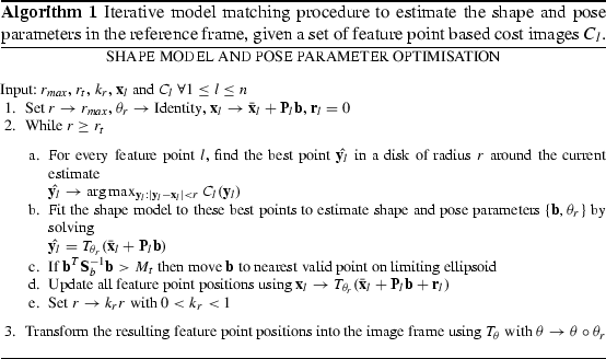
 of the current position in each cost image, applying the shape model and moving
  to nearest valid point on the limiting ellipsoid if the shape constraint in Eq. 2 is violated, updating all point positions using
  , and iterating whilst reducing
  . The initial disk radius
  was set to the search range
  , the search was terminated at
  pixels (in the reference image), and
  was set to
  . The optimisation is described in full in Algorithm 1.
3 Evaluation
A series of experiments was performed to optimise the various free parameters and options of the RFRV-CLM for application to the task of vertebral localisation in DXA images, and to compare the results to those achieved in [17] using AAMs. To facilitate this comparison, the same dataset and performance metrics were used. The dataset consisted of 320 DXA VFA images scanned on various Hologic (Bedford MA) scanners, obtained from: (a) 44 patients from a previous study [14]; (b) 80 female subjects in an epidemiological study of a UK cohort born in 1946; (c) 196 females attending a local clinic for DXA BMD measurement, and for whom the referring physician had also requested VFA (as approved by the local ethics committee). Manual annotations of 405 landmarks were available for each image, covering the thoracic vertebrae from T7 to T12 and the lumbar vertebrae from L1 to L4. Each of these vertebrae in each image was also classified by an expert radiologist into one of five groups (normal, deformed but not fractured, and grade 1, 2 and 3 fractures according to the Genant definitions [10]; see Fig. 1).
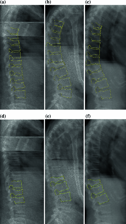

Fig. 1


Example DXA spinal images. a–c 405-point manual annotations. d–f Automatic annotation of the L2 vertebra (using the L1-L3 model), using the fully optimised, 2-stage RFRV-CLM. Example (a, d) shows grade 2 fractures on L2 and L3, (b, e) show a grade 3 fracture on L1, and (c, f) show a grade 3 fracture on L1 and a grade 1 fracture on L2
Stay updated, free articles. Join our Telegram channel

Full access? Get Clinical Tree


