). The correlation coefficient (r) for the TDIOF-derived circumferential strains compared to the tagged MRI-derived circumferential strains were 0.86 ( ). The comparison of TDIOF-derived and block matching speckle tracking and Horn-Schunck optical flow strain values using student t-test demonstrated superiority of TDIOF (95 % confidence interval,
  ).
).
1 Introduction
Cardiovascular Disease (CVD) is the leading cause of death in the modern world. The mortality rate associated with CVD was estimated to be 17 million in 2005 and continues to be ranked as the top killer worldwide. CVD is the result of under-supply of the cardiac tissue and can lead to malfunction of the involved myocardial territories and manifest as hypokinesia or akinesia. Several imaging methods such as X-ray CT, MRI, and Ultrasound have been used for visualization of the heart function. MRI and X-ray CT provide excellent spatial resolution but the cost and lack of wide-spread availability cause challenges in the clinical settings. Echocardiography is a popular technique for cardiac imaging due to its availability, ease of use, and low cost. Echocardiography shows the motion and anatomy of the heart in real time, enabling physicians to detect different pathologies. However, analysis of motion of the myocardium in echocardiographic images is based on visual grading by an observer and suffers from inter and intra-observer variability. To overcome the inter- and intra-observer variability, computerized image analyses can help by quantitatively interpreting the data. To that end, cardiac image processing techniques, mainly categorized as segmentation and registration, have been widely used for assessing the regional function of the heart [1–3]. To perform such analysis, two independent techniques, have been utilized; these are TDI (Tissue Doppler Imaging) and speckle tracking. TDI computes the tissue motion based on the Doppler phenomenon and is dependent on the angle of insonification. Speckle tracking, on the other hand,is an image processing method based on the analysis of the ultrasound B-mode or RF images. B-mode based algorithms are robust to the variation of the transducer angle but rely entirely on the properties of echocardiographic images which may be noisy or inaccurate. The physical principle underlying B-mode and TDI are to a large degree independent and therefore for myocardial motion estimation carry complementary information [4, 5].
Table 1
Description of some of the current methods used in motion detection in echocardiography images
Article | Output | Technique | Validation (# of subjects) |
|---|---|---|---|
Suhling et al. [6] | Motion | B-spline moments, optical flow | 2D dog (6), simulated images, phantom |
Yu et al. [7] | Motion | Maximum likelihood, spline based control points | 2D Dog (4), Sonomicrometry |
Paragios [8] | Endocardium, motion | Level set + learned shape-motion prior | 2D Human |
Hayat et al. [9] | Motion | Block matching | 3D echo, MRI |
Elen et al. [10] | Motion | Elastic registration | 3D human (normal: 3, patient: 1), simulated images |
Esther Leung et al. [11] | Motion | Optical flow and shape model | 3d echo |
Myronenco et al. [12] | Motion | Motion coherence by temporal regularization | 3D human, EB |
Duchateau et al. [13] | Motion | Diffeomorphic registration | 2D human (normal: 21, patient: 14), |
Bachner et al. [14] | Motion | fiber direction | 2D human, simulation, phantom |
Dydenco et al. [15] | Epicardium, motion | Regional statistics curve evolution | 2D Human, TDI |
Yan et al. [16] | Epicardium, motion | Finite element model | 3D human, implanted marker |
De Craene et al. [17] | Epicardium | Diffeomorphic B-spline free form deformation | 3D human (normal: 9, patient: 13) |
Ashraf et al. [18] | Motion | 3D Pig | Sonomicrometry |
Motion | Finite element model | 3D echo | |
Kleijn et al. [21] | Motion | Block Matching | 3D echo |
Many methods such as optical flow [6], feature tracking [7], level sets [8], block matching [9], and elastic registration [10] have been utilized for quantitative assessment of myocardial motion in B-mode images. Table 1 shows a description of some of the current methods used in motion estimation in echocardiographic images [6–21]. Suhling et al. [6] integrated rigid registration in an optical flow framework in order to detect myocardial motion from 2D echocardiographic images. B-spline moments invariants were applied to echo images to achieve invariance to the translation and rotation. The motion estimation algorithm was then applied to the B-spline moments of the image instead of the image intensity in a coarse to fine strategy and was validated using open chested dogs after ligation of a coronary artery. Additional validations were performed on simulation and phantom images. Ellen et al. [10] used elastic registration on 3D B-mode echocardiography images to extract myocardial motion and strain values. The method was validated using simulated and real ultrasoundimages. Esther-Leung et al. [11] proposed two different methods (1. model-driven, 2. edge-driven) for tracking the left-ventricular wall in echocardiographic images. Their approach was motivated by the fact that in echocardiography images, visibility of the myocardium depends on the imaging view; so the myocardium may be, partly, invisible to the beam. Their technique relied on a local data-driven tracker using optical flow applied to the visible parts of the myocardium and a global statistical model applied to the invisible parts. It was concluded that the shape model could render good results for both the visible and the invisible tissues in ultrasound images. Myronenco et al. [12] proposed the so-called Coherent Point Drift (CPD) technique for myocardial motion estimation, constraining the motion of the point set in the temporal direction for both rigid and nonrigid point set registration. A set of point distribution was computed based on endocardium and epicardium locations. The point set was modeled with a Gaussian mixture model (GMM). The GMM centroids were updated coherently in a global pattern using maximum likelihood to preserve the topological structure of the point sets. A motion coherence constraint was added based on regularization of the displacement fields. The purpose of regularization was to increase the motion smoothness.
Most of the motion estimation techniques developed thus far, are either based on TDI or B-mode. Recently, Garcia et al. [22] considered the combination of cardiac B-mode images and intra-cardiac blood flow data for computing the blood flow motion in the heart using continuity equation and mass conservation in polar coordinates. Their paper focused on the blood flow computation and did not consider the cardiac tissue displacements. Dalen et al. [23] and Amundsen et al. [24] previously combined TDI with speckle tracking by integrating TDI in the beam direction and speckle tracking in the direction lateral to the beam. However, this method discarded the speckle tracking data in the beam direction. The authors reported that they were unable to improve the motion estimation performance compared to speckle tracking techniques. In this paper, we propose integration of tissue Doppler and speckle tracking within a novel optical flow framework, we call TDIOF (Tissue Doppler Optical Flow). Our experimental results indicate that TDIOF outperforms both TDI and speckle tracking approaches.
The organization of the rest of the paper is as follows: in Sect. 2, we review the mathematical and algorithmic basis for the proposed method. Section 3 is a description of datasets used for validation of the proposed method. These include computational simulations, US data collected in a cardiac phantom, and in vivo data collected in patients recruited from the echocardiography laboratory at the Robley Rex VA Medical Center to our IRB-approved study. In Sect. 4, strain computations are discussed and, in Sect. 5, results from validation of the proposed method are described. Finally, in Sect. 6 we discuss observations related to TDIOF and our findings.
2 Methods and Materials
TDI and B-mode speckle tracking are different in both their physical underpinning and data type. In speckle tracking, tissue motion is determined from motion of speckles in Ultrasound images–typically, using a block matching approach applied to 2-D B-mode images [give references]. Although speckle tracking provides both components of the motion in the spatial domain, it is based on noisy B-mode images. TDI on the other hand only computes the velocity of tissue in one direction as moving towards (displayed as red) or away (displayed as blue) from the transducer. This means that the computed motion is the projection of the real motion in the direction of the transducer and therefore TDI is angle dependent. In this section, we first describe a novel energy minimization framework for estimation of myocardial motion from B-mode images which incorporates a velocity constraint from TDI.
The proposed method is based on optimization of three energy functions: (1) intensity constancy assumption, (2) velocity smoothness, and (3) similarity with Doppler data. The framework is minimized using an incremental algebra in method [25, 26] as described in Appendix A. In order to show the performance of TDIOF, it is compared to two popular motion detection techniques Horn-Schunck optical flow [27] and block matching [28] (Appendix B). Block matching is utilized in several commercial software platforms [29].
3 Validations
3.1 Simulated Computerized Phantom
Echocardiographic images are the result of the mechanical interaction between the ultrasound field and the contractile heart tissue. Previously, we reported on development and use of an ultrasound cardiac motion simulator [29]. In the current study, we utilized the COLE convolution based simulation technique reported in [30]. The significance of an Ultrasound cardiac motion simulator is the availability of both echocardiographic images as well as the actual ground-truth vector field of deformations.
Table 2
The 13 k-parameters of the Art’s kinematic model for left-ventricular deformation used in our cardiac US motion simulator
Non-rigid body motion | |
|---|---|
 | Radially dependent compression |
 | Left ventricular torsion |
 | Ellipticalization in long-axis (LA) planes |
 | Ellipticalization in short-axis (SA) planes |
 | Shear in x direction |
 | Shear in y direction |
 | Shear in z direction |
Rigid body motion | |
 | Rotation about x-axis |
 | Rotation about y-axis |
 | Rotation about z-axis |
 | Translation along x-axis |
 | Translation along y-axis |
 | Translation along z-axis |
A moving 3D heart was modeled based on a pair of prolate-spheroidal representations and used for the ultrasound simulation. The 3D forward model of cardiac motion was simulated using 13 time-dependent kinematic parameters of Arts et al. [30] (see Table 2). The evolution of the 13 kinematic parameters was previously derived by Arts following a temporal fit to actual location of tantalum markers in a canine heart [31]. In Arts’ model, seven time-dependent parameters are applied to define the ventricular shape change, torsion, and shear while six parameters are used to model the rigid-body motions. To simulate the Ultrasound imaging process, scatterers were randomly distributed in the simulated LV wall and the motion prescribed by Arts’ model was used to move the ultrasound scatterers. To determine Ultrasonic B-mode intensities, the COLE method was used [30]. COLE is an efficient convolution-based method in the spatial domain, producing US simulations by convolving the segmental PSF (point spread function) with the projected amplitudes of the scatterers [29] with the segmental PSF derived using Field II [30, 32]. In order to model the Doppler Effect, the frequency of the RF signal was shifted in the frequency domain based on the attributed ground truth motion vector and mixed with additive Gaussian noise. If the velocity of the particle is  , ultrasound velocity is
  , and transducer frequency is
  , then the frequency shift is:

The resolution of the first simulated sequence was 0.1 mm/pixel for both B-mode and TDI images and included 14 mid-ventricular temporal frames in the axial orientation. In order to analyze the robustness of the method to noise, another set of simulated images were produced by adding Gaussian noise of 1.12 db to the noise-less data
, ultrasound velocity is , and transducer frequency is , then the frequency shift is:(1)
3.2 Physical Cardiac Phantom
As described in [30], a physical cardiac phantom was built in-house, suitable for validation of echocardiographic motion estimation algorithms. Here, a brief description of this phantom is provided. To manufacture the phantom, a cardiac computerized model was used to build an acrylic based cardiac mold. A 10 % solution of Poly Vinyl alcohol (PVA) and 1 % enamel paint were used as the basic material. PVA has the ability to mimic cardiac elasticity, ultrasound and magnetic properties. The solution was heated up to 90  C. Consequently, it was poured into the cardiac mold and gradually exposed to the temperature of
 C until it froze. The mold and the solution were kept in that temperature for 24 h. Finally, the mold and the frozen gel were gradually exposed to the room temperature. At this point, the normal heart phantom has passed one freeze-thaw cycle.
C. Consequently, it was poured into the cardiac mold and gradually exposed to the temperature of C until it froze. The mold and the solution were kept in that temperature for 24 h. Finally, the mold and the frozen gel were gradually exposed to the room temperature. At this point, the normal heart phantom has passed one freeze-thaw cycle.An additional model consisting of the left and right ventricles but with a segmental thin wall in the LV was used to build an additional mold for a pathologically scarred heart. The thinner wall was designed to mimic an aneurysmal, dyskinetic wall. Three PVA-based inclusions were separately made as a circle; slab and cube using nine, six and three freeze-thaw cycles respectively. Each freeze-thaw cycle decreases the elasticity of the heart mimicking scarred myocardium. The attenuation of the PVA and speed of sound increase after each freeze-thaw cycle.The cylindrical, slab like and cube like objects were placed in the mold in different American Heart Association cardiac segments [33]. Subsequently, the PVA solution was added to fill the rest of the space in the mold. After one freeze-thaw cycle, the abnormal heart consisted of a background of normal texture with one freeze-thaw cycle plus three infarct-mimicking inclusions having 10, 7 and 4 freeze-thaw cycles. The speed of sound in PVA is 1527, 1540, 1545, and 1550 m/s and ultrasound attenuation is 0.4, 0.52, 0.57, and 0.59 db/cm for 1, 4, 7 and 10 freeze-thaw cycles. The parameters of the synthetic phantom was adjusted based on the previous phantom studies [34].
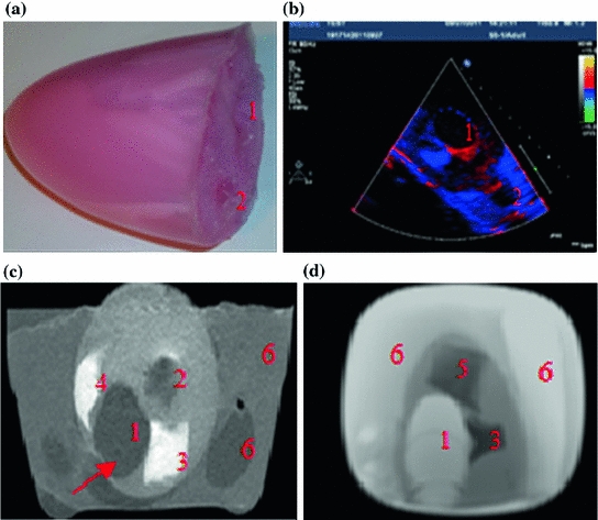
A mediastinal phantom that provides the ability to acquire trans-esophageal images was manufactured using another mold. A solution of 50 % water and 50 % glycerol was used to mimic the blood. Finally, a syringe was used to manually force the fluid inside and outside the phantom for contraction and expansion. The enamel paint particles are robust scatterers and can generate reliable markers on the B-mode image. Since each marker is not restricted to just one pixel, the center of the mass of each manually segmented marker is considered as landmark. The displacements of the landmarks are compared to the computed motion field for the validation purposes. Figure 1 shows the cardiac phantom and the acquired phantom images using ultrasound and MRI.
3.3 Patient Studies
Two separate sets of data were utilized for in vivo validations (sets A and B). Set A contained 15 patients and was used for manual tracking validation. Set B was a joint echo and tagged MRI set and was used for both manual tracking and comparison with tagged MRI (as will be discussed in Sect. 3.3.2) (Fig. 2).
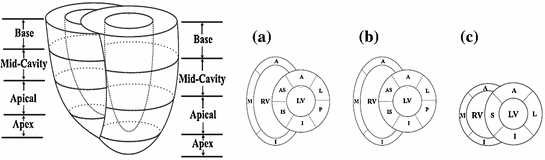
Fig. 2
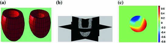
a A picture of the two-chamber model. b TDI image of the moving phantom during balloon inflation. c A static slice of the phantom using T1 weighted FFE. The arrow points to the aneurysm (the thin ventricular wall). d A static slice of the phantom using balanced FFE (1 LV, 2 RV, 3 cylindrical inclusion, 4 slab-like inclusion, 5 cube like inclusion, 6 mediastinum and mediastinal structures)
3.3.1 Set A: Echocardiography Studies
Data from fifteen subjects who had already undergone echocardiographic imaging as part of their diagnostic evaluation were deidentified and transferred to the laboratory following IRB approval. The data included 13 male, 4 female, average age  , consisting of hypertension (8 cases), Coronary Artery Disease (4 cases), Left Ventricular Hypertrophy (4 cases), Congestive Heart Failure (1 case), Chronic Obstructive Pulmonary Disease (2 cases), Diabetes Mellitus (2 cases) and smokers (1 case). 2D echocardiography (short-axis, long-axis, four-chamber, two-chamber B-mode with TDI. At the University of Louisville Hospital’s echocardiography laboratory, Echocardiographic images are acquired with a commercially available system (iE33, Philips Health Care, Best, The Netherlands) using a S5-1 transducer (3 MHz frequency) and the operator is free to change the gain and filter as needed. The full data set included two-chamber, three-chamber, four-chamber, and long-axis views.
, consisting of hypertension (8 cases), Coronary Artery Disease (4 cases), Left Ventricular Hypertrophy (4 cases), Congestive Heart Failure (1 case), Chronic Obstructive Pulmonary Disease (2 cases), Diabetes Mellitus (2 cases) and smokers (1 case). 2D echocardiography (short-axis, long-axis, four-chamber, two-chamber B-mode with TDI. At the University of Louisville Hospital’s echocardiography laboratory, Echocardiographic images are acquired with a commercially available system (iE33, Philips Health Care, Best, The Netherlands) using a S5-1 transducer (3 MHz frequency) and the operator is free to change the gain and filter as needed. The full data set included two-chamber, three-chamber, four-chamber, and long-axis views.3.3.2 Set B: Echocardiography-MRI Studies
The prospective protocol for patient selection and imaging was approved by the Institutional Review Board of the Robley Rex Veterans’ Affairs Medical Center, and a written informed consent was obtained from patients. Eight male subjects were prospectively recruited to the study with average age  The subjects included hypertension (5 cases), Coronary Artery Disease (2 cases), Congestive Heart Failure (1 case), Chronic Obstructive Pulmonary Disease (1 case), Diabetes Mellitus (3 cases) and smokers (4 cases).The imaging protocol included a primary 2D echocardiography including short-axis, long-axis, three-chamber, four-chamber and two-chamber B-mode and TDI imaging as well as simultaneous B-mode/TDI imaging (two-chamber, three-chamber, four-chamber, long-axis). At the Robley Rex Veterans Affair Medical Center’s echocardiography laboratory, Echocardiographic images are acquired with an iE33 commercial echocardiography system (Philips Health Care, Best, The Netherlands) using a S5-1 transducer (3 MHz frequency) and the operator is free to change the gain and filter as needed.
The subjects included hypertension (5 cases), Coronary Artery Disease (2 cases), Congestive Heart Failure (1 case), Chronic Obstructive Pulmonary Disease (1 case), Diabetes Mellitus (3 cases) and smokers (4 cases).The imaging protocol included a primary 2D echocardiography including short-axis, long-axis, three-chamber, four-chamber and two-chamber B-mode and TDI imaging as well as simultaneous B-mode/TDI imaging (two-chamber, three-chamber, four-chamber, long-axis). At the Robley Rex Veterans Affair Medical Center’s echocardiography laboratory, Echocardiographic images are acquired with an iE33 commercial echocardiography system (Philips Health Care, Best, The Netherlands) using a S5-1 transducer (3 MHz frequency) and the operator is free to change the gain and filter as needed.Following Ultrasound imaging, cine and tagged MRI data were collected in all subjects. Tagged MRI data acquisition was performed using Philips Achieva, TFE/GR sequence, TE/TR 2/4 ms, Flip Angle 15, spatial resolution  mm, slice thickness 8 mm, and spatial size
 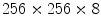 pixels. In all subjects, both echocardiography and MR imaging were performed within two hours to decrease any confounding events that could cause discrepancy between wall motion studies in echocardiography and MRI. MRI was performed immediately after the echocardiography. In order to ensure that the B-mode and TDI images were matched, B-mode and TDI images were simultaneously acquired. Additionally, subjects were asked to hold their breath during data collection.
mm, slice thickness 8 mm, and spatial size pixels. In all subjects, both echocardiography and MR imaging were performed within two hours to decrease any confounding events that could cause discrepancy between wall motion studies in echocardiography and MRI. MRI was performed immediately after the echocardiography. In order to ensure that the B-mode and TDI images were matched, B-mode and TDI images were simultaneously acquired. Additionally, subjects were asked to hold their breath during data collection.3.4 In-Vivo Comparison of TDIOF-Derived Strains with Strains from Tagged MRI
Tagged MRI [35] is known to provide highly accurate displacement fields in the systolic portion of the cardiac cycle while the tags last. We analyzed the strain field in echocardiography and tagged MR images of slices similar in location in the two modalities in set B. In selecting corresponding slices, qualitative anatomical landmarks such as the papillary muscles and cardiac contours as well as cine MRI images were utilized. Anatomical landmarks such as endocardial shape and papillary muscle were used to locate the appropriate short axis sections of the heart. The recently proposed SinMod technique [36] was then used to derive displacements from tagged MRI data in the first few systolic phases of the cardiac cycle, while the tags persisted. SinMod is an automated motion estimation technique for tagged MRI that models the pixels as a moving sine wavefront.Since no pixel to pixel mapping between echo and MR images was known, the ventricular geometry from 2-D echo and tagged MRI was divided into 17 segments following the American Heart Association’s recommendations. Subsequently the averaged Lagrangian strain for each of the 17 heart segments were compared between the two modalities. Since the frame rate of echo and MRI is not the same and the heart rate may change, it was necessary to align the images in the temporal dimension. This was done by spline interpolation of the measured strain data in the time domain.
4 Strain Analysis
Strain is a measure of deformation of the cardiac tissue. With  representing the identity matrix, the Lagrangian strain tensor at a given myocardial point and for a specific time point can be expressed as:
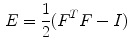
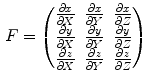
where the elements of the deformation gradient tensor, F, are:
while  represents the spatial coordinates in the undeformed coordinates (typically taken to be the end-diastolic frame), and
  is the accumulated motion vector at the corresponding spatial location relative to the undeformed state . For the echocardiography data, the reference frame for the strain computation was considered to be the end diastolic frame and was selected based on ECG trigger. The deformation field was then computed between each two frames and was added to the motion field from the previous frame in order to measure the accumulated deformation and strain . Since the deformation field of the consecutive frames do not represent the motion of the same pixels, spline interpolation was used to align the deformation fields. For the tagged MRI data, the end-diastolic frame was always the first acquired image which is collected immediately after the R-wave trigger.
representing the identity matrix, the Lagrangian strain tensor at a given myocardial point and for a specific time point can be expressed as:(2)
(3)
represents the spatial coordinates in the undeformed coordinates (typically taken to be the end-diastolic frame), and is the accumulated motion vector at the corresponding spatial location relative to the undeformed state . For the echocardiography data, the reference frame for the strain computation was considered to be the end diastolic frame and was selected based on ECG trigger. The deformation field was then computed between each two frames and was added to the motion field from the previous frame in order to measure the accumulated deformation and strain . Since the deformation field of the consecutive frames do not represent the motion of the same pixels, spline interpolation was used to align the deformation fields. For the tagged MRI data, the end-diastolic frame was always the first acquired image which is collected immediately after the R-wave trigger.The normal strain in the direction of the unit vector n can be calculated from the Lagrangian strain tensor through the quadratic form  , where n is a unit vector and can point to any direction on the unit sphere. Due to the geometry of the left ventricle, the normal strains are usually calculated in radial, circumferential, and longitudinal directions.
, where n is a unit vector and can point to any direction on the unit sphere. Due to the geometry of the left ventricle, the normal strains are usually calculated in radial, circumferential, and longitudinal directions.Regional analysis is performed on 17 American Heart Association (AHA) prescribed segments. Figure 7 shows the different segments. The acronyms stand for antero-septal (AS), anterior (A), lateral (L), posterior (P), inferior (I), and infero-septal (IS). For a review of topics related to determination of strain from cardiac images, the reader is referred to [35, 37, 38].
5 Results
As noted in Sect. 3, TDIOF was applied to three different datasets: simulated images, data collected in a physical phantom, and in vivo data (both set A and set B). To further elucidate the effect of the Doppler term, results from TDIOF were compared to Horn-Schunck (HS) optical flow (beta = 0 in Eq. (A.11)) and block-matching (BM) (see Appendix) with the latter being the basis for most commercial speckle tracking methods [13]. Since the performance of each technique depends on the parameters of the method, it was necessary to optimize the parameters. Based on simulated images, an exhaustive search was performed over the parameters of TDIOF, HS optical flow, and BM speckle tracking method (a large range was considered for each parameter) and the best values were selected experimentally. To analyze the performance of the techniques with different parameter settings, simulated images were compared to the next simulated frame after being warped using the estimated motion field. Relative mean absolute error was used for the comparison. Relative mean absolute error was computed as 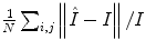 ; where
  and
and  are the first and subsequent warped images, and
  is the total number of points. Figure 3 shows the performance of the TDIOF technique using different parameters. The methods were then applied to all the datasets using the resulting parameters: number of scales for multiscale implementation:
  (smoothness weight):
  (TDI similarity weight): 0.001, and
  (penalizer parameter): 0.1. The parameters for the HS technique were set as follows: number of scales 5, and smoothness weight 2000.
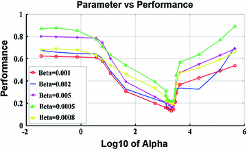
; where and are the first and subsequent warped images, and is the total number of points. Figure 3 shows the performance of the TDIOF technique using different parameters. The methods were then applied to all the datasets using the resulting parameters: number of scales for multiscale implementation: (smoothness weight): (TDI similarity weight): 0.001, and (penalizer parameter): 0.1. The parameters for the HS technique were set as follows: number of scales 5, and smoothness weight 2000.Fig. 3
Performance of TDIOF using different parameters based on relative mean absolute error: X-axis is shown with a logarithmic scale in order to report a wide range of parameter settings. The performance of TDIOF is plotted versus smoothness coefficient for different TDI similarity coefficients ( ). Changes of performance is evident when smoothness parameter (
 ) changes. As seen from the plots, performance was more dependent on the smoothness and insensitive to the scale for the TDIOF term
). Changes of performance is evident when smoothness parameter () changes. As seen from the plots, performance was more dependent on the smoothness and insensitive to the scale for the TDIOF term5.1 Validations on Simulated Images
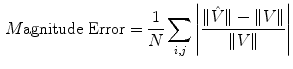
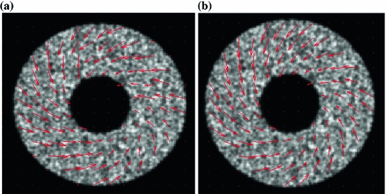
The simulated 3D cardiac model built based on Arts’ et al. [31] is shown in Fig. 4a. The deformation shown in the figure is that of a systolic motion. The 3D B-mode image deformation was computed based on [29] and was shown in Fig. 4b. Figure 4c shows the computed TDI using the simulated sequence—the red colors represent motion towards the transducer and the blue colors represents motion away from the transducer. Figure 5 shows application of TDIOF to simulated data and comparison with ground truth. Angular and magnitude error metrics were used for validation of the proposed technique as stated in Eqs. (4) and (5):
(4)
(5)
Fig. 4
a Simulated cardiac model in diastole and systole. b A 3D simulated B-mode image based on COLE. c The computed tissue Doppler image using the simulated sequence
Fig. 5
a Results of TDIOF from a mid ventricular section of the 3D simulated echo data. b Ground truth motion field
where and
and  are the true and estimated displacement vectors and
  is the total number of vectors.
and are the true and estimated displacement vectors and is the total number of vectors.Table 3


TDIOF versus HS optical flow and BM speckle tracking when applied to simulated images
Related posts:
Stay updated, free articles. Join our Telegram channel
Full access? Get Clinical Tree
