Optimizing the breast magnetic resonance imaging (MRI) protocol requires many decisions to be made about image acquisition techniques, types of pulse sequences, and sequence parameters used to control image quality and acquisition speed. Fundamental trade-offs exist among spatial resolution, acquisition speed, and signal-to-noise ratio, and these trade-offs must be understood in order to optimize quality and speed consistent with diagnostic goals. Image contrast is controlled by the pulse sequence and its acquisition parameters through manipulation of the magnetic resonance (MR) signal from hydrogen protons in tissue. To understand how acquisition techniques, pulse sequences, and pulse sequence parameters can be used to optimize the breast MRI protocol, it is important to first understand the fundamentals of MRI. This chapter will begin with a review of these fundamentals, followed by information on pulse sequences and acquisition techniques. These elements will be summarized with recommendations for optimizing the overall breast MRI protocol.
Fundamentals of Magnetic Resonance Imaging
Protons and the Main Magnetic Field
The strong magnetic field associated with the MR scanner is typically called the main magnetic field or the B 0 (”B zero”) field. This B 0 field typically points in a direction called the longitudinal direction or z direction ( Figure 2.1 ). The plane perpendicular to this direction is defined by the x and y directions, and is called the transverse plane (see Figure 2.1 ). The z direction is horizontal for high field strength cylindrical bore scanners.

Protons act like tiny bar magnets and align with or against the longitudinal direction when brought in the vicinity of the strong magnetic field of the MR scanner. Because some protons are aligned with B 0 and some are aligned in the opposite direction, the small magnetic fields associated with many of these protons will cancel out. A proportion of protons remains, aligned in the longitudinal direction and resulting in a net magnetization. This net magnetization is manipulated by the pulse sequence and becomes the MR signal that is measured by the MR coils, producing the tissue contrast in the acquired images.
Protons also precess when in the vicinity of a strong magnetic field. This precession (like the precession of a child’s spinning top) occurs at a certain frequency, ω 0 , determined by the Larmor equation, ω 0 = B 0 × γ (gamma is a constant called the gyromagnetic ratio).
Radiofrequency Pulse
Radiofrequency (RF) energy is transmitted by the RF coil (located in the bore of the scanner). This transmitted RF energy can be turned on and off and is called an RF pulse. If the frequency of this RF pulse matches the precessional frequency of the protons, ω 0 , resonance occurs and the protons will absorb some of this energy. Recall that the net magnetization is aligned in the longitudinal direction. This net magnetization is also called longitudinal magnetization.
As energy is absorbed, the net magnetization rotates away from the longitudinal direction. How far the net magnetization rotates depends on the strength and duration of the RF pulse. If an RF pulse is provided that rotates the net magnetization to the transverse plane, then a 90° RF pulse was used ( Figure 2.2 ). If the net magnetization rotates to the – z direction, then a 180° RF pulse was used.

After the RF pulse turns off, the protons begin to release energy in a process called relaxation. There are two types of relaxation, called T1 relaxation and T2 relaxation.
T1 Relaxation and Contrast
Let’s assume a 90° RF pulse is used to rotate the net magnetization to the transverse plane. The net magnetization is no longer pointing in the longitudinal direction, but slowly the protons will begin to realign in this direction of the main magnetic field. After a “long” time (several seconds), most of the magnetization will have realigned in the longitudinal direction. The realignment in this direction is called T1 relaxation or longitudinal relaxation. The amount of magnetization that has realigned in this direction can be shown on a graph ( Figure 2.3 ). The realignment occurs at a rate that is characterized by a time constant, T1, called the T1 relaxation time.

A key point is that the protons or magnetization associated with different tissues will realign with the longitudinal direction at different rates ( Figure 2.4 ) and thus will have different T1 relaxation times. This is the source of contrast in T1-weighted images, in which tissues with shorter T1 relaxation times will be brighter than tissues with longer T1 relaxation times. The T1 relaxation time of fluid is longer than that for fibroglandular tissue. Thus cysts are darker than fibroglandular tissue on T1-weighted images. The T1 relaxation time of a tissue depends on the strength of the magnetic field surrounding that tissue. T1 relaxation times for various breast tissues at 1.5 tesla (T) and 3.0 T magnetic field strengths are listed in Table 2.1 .

| Tissue | 1.5 T | 3.0 T | ||
|---|---|---|---|---|
| T1 | T2 | T1 | T2 | |
| Fat | 250 ms | 60-80 ms | 423 ms | 154 ms |
| Normal fibroglandular tissue | 700 ms | 60-80 ms | 1680 ms | 71 ms |
| Cyst | 3000 ms | 300 ms | — | — |
| Lesion | 800-1000 ms | 80-100 ms | — | — |
| Enhanced lesion | 200-400 ms | — | — | — |
T2 Relaxation and Contrast
Let’s assume again that a 90° RF pulse has just been applied. As before, the net magnetization rotates from the longitudinal direction to the transverse plane. This magnetization in the transverse plane is called transverse magnetization. T2 relaxation is a simultaneous and independent process involving the magnetization just rotated to the transverse plane. Recall that this magnetization is made up of many different protons. The protons are all precessing, but because of several factors (mentioned below) these protons are not all precessing at the same frequency. The slightly different frequencies of the protons cause the transverse magnetization to dephase ( Figure 2.5 ). The transverse magnetization ultimately provides the actual MR signal that is measured by the receive RF coils. Just after the 90° RF pulse, when the protons are all in-phase, the MR signal is strong. As the transverse magnetization begins to dephase, the MR signal decreases as shown in Figure 2.5 .

Several factors make the protons precess at slightly different frequencies. These factors (which will not be discussed in detail here) include spin-spin interactions, magnetic field inhomogeneities, chemical shift, and magnetic susceptibility. The dephasing due to each of these can be reversed—except for spin-spin interactions—using an SE technique as discussed below. The dephasing due to spin-spin interactions cannot be reversed. The decrease in signal due only to spin-spin interactions occurs at a rate that is characterized by a time constant, T2, called the T2 relaxation time. The rate of decrease in signal due to all factors is characterized by the T2∗ relaxation time.
A key point is that different tissues will have different T2 relaxation times, as shown in Figure 2.6 . This is the source of contrast in T2-weighted images, in which tissues with longer T2 relaxation times will be brighter than tissues with shorter T2 relaxation times. Thus cysts are brighter than fibroglandular tissue on T2-weighted images. The T2 relaxation time of a tissue is a characteristic of that tissue. T2 relaxation times for various breast tissues are listed in Table 2.1 . Knowledge of T1 and T2 relaxation times is important for understanding how to optimize contrast in breast MR images.

Understanding Pulse Sequences
Pulse sequences take advantage of the different relaxation times (T1 and T2) of various tissues and manipulate the net magnetization in a way that produces desired image contrast. Several different types of pulse sequences exist, including spin echo, fast spin echo (or turbo spin echo), and gradient echo. Each pulse sequence has several parameters that can be adjusted to control contrast, spatial resolution, scan time, signal-to-noise ratio, and so on.
An aid to understanding the various types of pulse sequences is found in the use of diagrams that display the main features of the pulse sequence. Basic diagrams will be shown with each type of pulse sequence below. The features of a pulse sequence will be described using the spin echo pulse sequence as an example. Figure 2.7 shows the pulse sequence diagram for the spin echo pulse sequence. Time moves across horizontally. The top line shows the placement in time of RF pulses. A 90° and a 180° RF pulse are shown. The second line displays the transverse magnetization or MR signal that can be measured by the receive RF coil. The 90° RF pulse produces transverse magnetization that dephases because of the processes mentioned above, and the 180° pulse is used to reverse transverse magnetization, which reverses the effects of everything except spin-spin interactions, and produces the “spin echo” as shown.

Lines 3 to 5 of Figure 2.7 show gradient magnetic field operation, which is used to divide the MR signal into image slices and pixels (or voxels). Three gradients are responsible for splitting the signal into three orthogonal directions. These gradients are called the slice select gradient, frequency-encoding gradient, and phase-encoding gradient. The slice select gradient is turned on during the 90° and 180° RF pulses (in two-dimensional [2-D] acquisition mode) and is responsible for exciting the protons in the slice of interest so that signal comes only from these protons.
The frequency-encoding gradient is turned on during signal acquisition of the SE and is responsible for dividing up the signal along the frequency-encoding direction. The echo is sampled at this time, and these data are entered into one line of “k-space,” which stores the raw data for reconstruction into images. The pulse sequence must be repeated a number of times to collect all the information needed to produce an image. For a 256 by 256 image this pulse sequence would be repeated 256 times.
The phase-encoding gradient is adjusted each time the pulse sequence is repeated and is responsible for placing data in each line of k-space. The time from the 90° RF pulse to the center of the SE is the echo time or TE (see Figure 2.7 ). The time that it takes to run the pulse sequence one time is the repetition time or TR. TE and TR are user-selectable parameters of a pulse sequence that are used to determine image contrast.
Contrast Formation
To illustrate the importance of TE and TR we turn back to graphs showing T1 and T2 relaxation ( Figure 2.8 ), which occur simultaneously and independently. The height of these curves is related to the tissue signal (image brightness) measured during the pulse sequence; the vertical separation is related to the contrast between tissues. TR is used to select the amount of T1 weighting on the curves labeled T1 Relaxation, and TE is used to select the amount of T2 weighting on the curves labeled T2 Relaxation.

Placing TR at position A in Figure 2.8 maximizes T1-related contrast by taking advantage of the large separation in T1 relaxation for these tissues. Placing TR at position B minimizes T1 contrast by imaging when the difference in relaxation for these tissues is minimal.
Placing TE at position C minimizes T2 contrast by imaging when T2 relaxation for these tissues is not very different. Placing TE at position D maximizes T2-related contrast by taking advantage of the large separation in the T2 relaxation for these tissues.
Thus, to obtain T1-weighted contrast, TE and TR would be placed as shown in Figure 2.9 to maximize T1 effects and minimize T2 effects. To obtain T2-weighted contrast, TE and TR would be placed as shown in Figure 2.10 to maximize T2 effects and minimize T1 effects. Positioning TE and TR to minimize both T1 and T2 relaxation effects ( Figure 2.11 ) results in spin density contrast, in which image brightness is related to the density of hydrogen protons in the tissue. An important part of optimizing the breast MRI protocol includes optimizing the pulse sequence to obtain the maximum contrast possible. This is done primarily through optimizing the values of TE and TR.


MR contrast agents using gadolinium can be used to increase the image brightness of tissue and lesions that take up the contrast material. Gadolinium has seven unpaired electrons that affect the magnetic field near the gadolinium atoms and shorten the T1 and T2 relaxation times of nearby tissue. Because a tissue with a shorter T1 will be brighter than adjacent tissue with longer T1, a lesion that has taken up gadolinium will be brighter than surrounding tissue. Because the change in the rate of T1 relaxation is more significant than the change in the rate of T2 relaxation, contrast injected imaging is primarily done with T1-weighted imaging. Additional information regarding the fundamental physics of MR can be found in the suggested readings.
Fundamental Trade-offs
Fundamental trade-offs exist among image resolution, scan time, and signal-to-noise ratio. Managing these trade-offs is critical when optimizing the breast MRI protocol. Given a minimum adequate level of signal, high resolution imaging is typically achieved at the expense of longer scan time. On the other hand, if reduced scan time is a priority, this is often accomplished at the expense of resolution.
Resolution
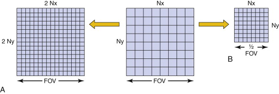
The spatial resolution of an imaging study is controlled by several acquisition parameters in the pulse sequence. Spatial resolution is directly related to pixel size and slice thickness, which together make up the size (volume) of an image voxel. Spatial resolution improves as voxel volume decreases, that is, as pixel size and/or slice thickness decrease. Smaller pixel size (area) provides better in-plane resolution. Pixel size in one direction is equal to the field of view (FOV) in that direction divided by the number of pixels in that direction. The pixel size in the “ x ” direction, P x = FOV x / N x . As shown in Figure 2.12 , increasing the number of pixels while keeping FOV the same (A) or decreasing the FOV while keeping the number of pixels the same (B) will decrease pixel size and improve spatial resolution.