Measuring and modeling the mechanical properties and behavior of materials is an important part of many fields of science. From improving the design of roads and buildings to creating artificial tissues and organs, knowledge of the mechanical properties of the individual components of a system and of the system as a whole are critical for the adequate performance of the final structure. Considerable research has been involved in the development of artificial tissues and organs, such as the heart, lung, liver, skin, and cartilage [11–14]. In some cases, the primary goal is to replicate the function of the original organ (e.g., the artificial heart). However, in other cases, reproducing the mechanical properties of the original tissue is equally important because reproducing the mechanical response of the tissue under physiologic conditions will increase the chance that the patient will be able to return to normal activities with a normal range of motion and function. Therefore, understanding the mechanical properties of healthy and diseased tissue is important not only for diagnosing and characterizing a disease, but also for understanding and monitoring tissue function.

A number of mechanical tests exist for measuring the static and dynamic properties of materials (e.g., indentation, impact, creep, and torsion tests) [15–18]. These mechanical tests involve applying a known force (or stress) to the material and measuring the resulting displacement (or strain) of the material. For example, in an indentation test, a small probe is used to deform a small sample of a material. By measuring the amount of force that is being applied by the probe and the amount of deformation of the sample that results, material properties such as the Young’s modulus, another indicator of material stiffness, can be determined. The response of a material during a particular test will depend on several mechanical properties, including anisotropic, nonlinear, thermal, geometric, composite, plastic, viscous, flow, and elastic effects. By carefully controlling the design of these experiments, and by making simplifying assumptions about the characteristics of the material and the applied stresses, the results of these measurements can be interpreted in meaningful ways (e.g., [17–31]).

A typical set of assumptions made when measuring the mechanical properties of a material is that of an infinite, homogeneous, linear, viscoelastic material [9, 32–34]. This set of assumptions significantly reduces the complexity of the mathematical relationship between the applied stresses and the resulting strains, and also reduces the number of unknown material properties that have to be determined to characterize the material. By assuming the material to be infinite, the impact of certain boundary conditions and boundary effects can be ignored. Assuming the material to be homogeneous (at least within a small region where data processing is performed) means only one set of material parameters needs to be considered and changes in the mechanical properties in space are negligible. Treating the material as linearly viscoelastic means that the strain of the material is linearly related to the applied stresses, though the response may change depending on the rate at which the stress is applied. Clearly, the validity of assumptions such as these must be reconsidered with every application because different materials and different experimental setups will have different characteristics.

Under the above assumptions, a fully anisotropic material may contain 21 independent quantities that would have to be known in order to fully characterize the material. The number of unknowns can be reduced by assuming that the material has certain symmetries. In a transversely isotropic material, the material is considered to have one preferential direction in which the response of the material is different from the response in the orthogonal directions. For example, in muscle, the response of muscle tissue along the direction of the muscle fibers to a particular stress will be different than the response of the tissue to a similar stress applied across the muscle fibers. Transversely isotropic materials can be described using as few as three parameters. Another common symmetry assumption is that the material under investigation is isotropic, and thus responds equally to stresses in any direction. An isotropic material only requires two quantities to describe its mechanical behavior, and several such quantities have been defined to aide in the description of the behavior of isotropic materials. These quantities include the Lamé parameters λ and μ (μ also being called the shear modulus), Poisson’s ratio (ν), Young’s modulus (E), the bulk modulus (K), and the P-wave modulus (M). Knowledge of any two of these quantities allows for the calculation of the others. For example, by knowing the shear modulus and Poisson’s ratio, the others can be calculated as

To facilitate the analysis of the mechanical response of different types of materials under different loading conditions, the equations relating the stresses and strains can be expressed in different forms [9]. One such technique is to study the frequency-domain equations of motion for an infinite, isotropic, homogeneous, linear, viscoelastic material experiencing time-harmonic motion (such as a periodic deformation of tissue) [33]. These equations can be written as a set of complex-valued, coupled differential equations as
where ρ is the density of the material, ω = 2πf, f is the frequency of the harmonic motion, and U(r, f) is the vector displacement of the material at the position r. These equations can be used to show that, under the above assumptions, the response of the material is to propagate shear waves and longitudinal waves. Longitudinal waves have the property that the direction of the displacement of the material is in the same direction as the direction of wave propagation. Shear (or transverse) waves have the property that the displacement is perpendicular to the direction of wave propagation. The wave speed of the shear and longitudinal waves (c _S and c _L , respectively) can be written as
where |μ|, ℜ(μ), and ℑ(μ) indicate the magnitude, real part, and imaginary part of the complex-valued quantity μ, respectively.

It has been shown that the shear wave speed can vary significantly between different healthy and diseased tissues, from less than 1 m/s to over 100 m/s [10, 35, 36]. However, the longitudinal wave speed for most soft tissues is about 1,540 m/s and does not vary significantly between different types of tissue. Therefore, assessing the shear modulus and the shear wave speed has been the primary target for researchers trying to use the mechanical properties of tissue as indicators of disease.

Over the last 20 years, a number of imaging techniques have been developed to obtain information about the mechanical properties of tissue in vivo. Figure 2.2 provides a summary of the literature published on the topic of elasticity imaging over this time. This figure reflects the result of searching for “elastography” in the PubMed and Web of Knowledge databases for each publication year, ignoring false hits and conference abstracts, and differentiating the articles based on the primary imaging technique used or discussed. The imaging techniques, which will be discussed in more detail below, were crudely classified as [1] any ultrasound elasticity or strain imaging, [2] any phase-based MR elasticity or strain imaging, and [3] any other technique, including optical coherence tomography, X-ray, and MR tagging. While not an exhaustive or definitive search, the point of this figure is to indicate the rapid growth that the field of elasticity imaging has experienced, even in just the last 5 years in which the number of publications has doubled. This reflects the growing interest in the field and the rapid development of elasticity imaging techniques and applications.

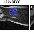
Imaging the elastic properties of tissue involves several important steps. First, a static, transient, or harmonic force is applied to the tissue. Second, the resulting internal displacements of the tissue are measured. Third, the measured displacements are used to solve the equations of motion [e.g., Eq. (2.2)] that are assumed to model the behavior of the tissue to determine the mechanical properties of the tissue. Throughout the evolution of elasticity imaging, numerous approaches have been developed to accomplish each of the above steps, each with its own benefits and limitations. Figure 2.3 shows a classic phantom experiment used to demonstrate these elasticity imaging principles.

The process of producing tissue motion can be performed using both extrinsic and intrinsic sources. Classic examples of extrinsic sources of motion include the use of piezoelectric elements, electromechanical actuators, and pneumatically powered drums and tubes that are placed in contact with the body [37, 38]. The vibrations produced by these external devices propagate into the body and throughout the tissue of interest. In contrast, changes in blood and CSF pressure, as well as the motion of the beating heart, can serve as sources of intrinsic motion and can produce motion directly within tissue [39–43]. Focused-ultrasound techniques, such as using amplitude modulation or interfering ultrasound beams, have also been employed as an external source of vibration that is capable of producing motion directly within tissue [44–50].

Tissue displacement can be measured in vivo using a number of techniques, including ultrasound, MRI, X-ray, and optical methods. A number of ultrasound-based methods for measuring tissue motion have been used for elastographic imaging, including Doppler imaging and cross-correlation techniques [51–54]. These techniques have been used to image many different types of tissue, including muscle, skin, liver, breast, heart, prostate, and blood vessels. In Doppler-based ultrasound elasticity imaging, including “sonoelasticity,” local tissue vibrations due to dynamic deformations cause Doppler shifts in the ultrasound signal which are used to measure tissue velocity changes over time [55–58]. The Doppler information can be used to obtain images showing wave propagation through tissue from which shear wavelengths and wave speeds can be obtained, which can be used to derive the elastic properties of the tissue [56, 59]. This record of tissue motion can also be used to calculate displacement and strain, as in the speckle-tracking techniques below, or it can be used with an appropriate equation of motion to directly solve for quantitative tissue mechanical properties. In speckle-tracking ultrasound elastography techniques, repeated ultrasound acquisitions are obtained while tissue is undergoing quasistatic or dynamic deformations [40, 60–63]. Cross-correlation analysis comparing successive images allows for estimates of the tissue displacement between the two acquisitions. The measured displacements can then be used to calculate strain maps (qualitative images of tissue elasticity) which are used to characterize the tissue [64–67] or to track wave propagation through the tissue for purposes of calculating the wave speed, which relates to tissue stiffness [62, 63]. The transient elastography method, also called Fibroscan, has become a very popular technique for quickly assessing hepatic fibrosis in vivo and noninvasively [62, 68]. Ultrasound elastography using ultrafast imaging techniques perform speckle-tracking to measure tissue displacement, but use customized hardware to acquire and reconstruct images at an effective frame rate of about 5,000 images per second [46, 63]. This method can image steady-state and transient wave propagation with high temporal and spatial resolutions and can be used to estimate tissue mechanical properties, including anisotropic and nonlinear properties [69, 70]. The primary limitations of these techniques are those produced by the ultrasound imaging itself in that an acoustic window is required to get the ultrasound signal into the tissue, the tissue displacement can typically only be measured in one direction (along the direction of the ultrasound beam), and the measurement depth is limited by the attenuation and scattering of the ultrasound beam.

Optical elastography methods have also been developed which are similar to speckle-tracking and Doppler ultrasound elastography, but use light instead of ultrasound to measure the tissue motion [71–76]. The higher resolution achievable with optical elastography makes it desirable for applications such as vascular imaging. However, like its ultrasound counterpart, this technique can only image tissue through an appropriate optical window, it can only measure displacements along the direction of the light beam, and it has significant depth limitations because of the high optical scattering and attenuation properties of tissue. Elastography techniques using X-rays have focused on acquiring static or quasistatic anatomical images and either using closed-form solutions to mechanical models of tissue deformation assuming certain geometries to determine mechanical properties, or using finite-element methods to iteratively adjust the assumed mechanical properties of a model until the model of the tissue behaves like the observed tissue deformation [77–80]. The X-ray and optical elastography techniques have not been as well developed as their ultrasound and MR counterparts.

Numerous MRI techniques have been developed over the years for measuring tissue motion and for determining the mechanical properties of tissue. Several methods have been developed which use the technique of spatial modulation of magnetization (SPAMM) to modulate the longitudinal magnetization of tissue to produce banding or grid patterns in the MR images that move with the deformation of the tissue [81–84]. From the MR images, the deformation of the grid pattern can be determined and used to estimate the strain distribution throughout the tissue. These techniques have been used for assessing cardiac and skeletal muscle function as well as for studying intrinsic brain motion and models of traumatic brain injury [82, 85–90]. Like many of the speckle-tracking ultrasound and optical techniques, this technique only provides qualitative estimates of tissue mechanical properties unless additional assumptions are made about the tissue boundary conditions or the characteristics of the applied stresses. Another limitation of SPAMM techniques is that they typically require large-amplitude motion in order for the grid pattern to be tracked. While most SPAMM-based techniques produce in-plane grid patterns to measure tissue displacement, a similar approach using through-plane SPAMM tagging was developed in which the quasistatic compression of tissue can be used to produce strain-encoded images [91]. Because it does not actually track the motion of the SPAMM tags, this method is less computationally demanding than the conventional SPAMM technique, but it still only produces qualitative images of tissue mechanical properties.

In the SPAMM-based elastographic imaging techniques, tissue motion is calculated from a series of MR magnitude images. An alternative approach is to encode tissue motion into the phase of the MR signal. Normally, the magnetic field gradients used in MRI are used to determine the position of tissue that is assumed to be static. However, motion that occurs during these gradients will result in additional phase in the measured transverse magnetization according to
where φ(r ₀, t) is the motion-induced phase of tissue, originally at r ₀, at a time t after the creation of the transverse magnetization, γ is the proton gyromagnetic ratio, G(t) is the magnetic field gradient vector, and u(r ₀, t) models the motion of the tissue at r ₀ [92, 93]. This characteristic of the MR signal has been used for such applications as diffusion imaging, flow imaging, and compensating for flow artifacts [92–96].

Several MR elastography (MRE) techniques using phase-based motion encoding have been developed to measure the quasistatic and harmonic deformation of tissue. One of the MRE techniques developed involves the imaging of quasistatic tissue compression using a stimulated-echo MR acquisition [97–100]. Stimulated-echo MRE utilizes three RF pulses: the first RF pulse creates the transverse magnetization of the tissue while the tissue is in its initial state, the second RF pulse temporarily stores a portion of that signal as longitudinal magnetization while the tissue is deformed from its initial state (during the “mixing” time of the stimulated-echo sequence), and the third RF pulse returns the stored longitudinal magnetization to the transverse plane to be measured while the tissue is still in its deformed state. To determine the amount of motion that the tissue has experienced, motion-encoding gradient pulses are incorporated into the imaging sequence before and after the mixing time. For tissue that does not move during the mixing time, the effects of the motion-encoding gradients (MEG) cancel each other and no net phase shift is recorded. However, in regions where the tissue has moved, a phase shift will be recorded that is proportional to the amount of displacement that has occurred. Like the SPAMM technique, this record of the tissue displacement that is present in the MR images can be used to calculate the strain distribution within the tissue and to provide qualitative measures of tissue mechanical properties. To determine the tissue properties quantitatively, additional assumptions must be made about the boundary conditions and the stresses applied to the tissue.

An alternative form of MRE emerged from the desire to image the response of tissue to dynamic stresses [101, 102]. By using time-harmonic motion, equations of motion like Eq. (2.2) could be used to directly determine tissue mechanical properties, even without knowledge of the boundary conditions present during the acquisition. Early work showed that MR imaging sequences could be easily modified to be sensitive to periodic motion and that the properties of the acquisition could be tailored to enhance the sensitivity to motion at a particular frequency, or to yield broadband motion sensitivity, depending on the application [102–107]. Much like velocity encoding in MR vascular flow imaging, the motion sensitivity of MRE is accomplished by adding additional MEG into standard MR imaging sequences which encode additional phase into the MR images in accordance with Eq. (2.4). Examples of MR imaging sequences which have been modified for MRE include gradient-recalled echo (GRE), spin echo (SE), echo planar imaging (EPI), balanced steady-state free precession (bSSFP), spiral, and stimulated-echo sequences [101–103, 106, 108–113]. Examples of GRE and SE-EPI MRE pulse sequences are shown in Fig. 2.4. Also like vascular flow imaging, MRE acquisitions are often repeated with two different amplitudes for the MEG (as indicated by the dashed MEG in Fig. 2.4). These two datasets are then combined to increase motion sensitivity while removing static phase errors from the images. In most applications, the MRE phase data are considered to be directly proportional to the tissue motion, thus the phase data can be substituted for displacement in equations of motion, such as Eq. (2.2), to determine the tissue mechanical properties.

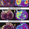
Because the tissue motion in dynamic MRE is dynamic, the imaging sequence and the motion must be synchronized so that the timing, or phase relationship, between the motion and MEG remains constant during the acquisition. Each phase image produced in this fashion (also called a “wave image”) is equivalent to imaging the dynamic displacement field at one instant in time. By changing the timing between the motion and MEG from one image acquisition to the next, multiple images (“phase offsets”) can be obtained which show the propagation of the displacement field over time. The time-domain data can then either be processed directly, or analyzed in the Fourier domain to isolate the motion occurring at specific frequencies. Besides continuous periodic vibrations, the propagation of transient impulses through tissue can also be imaged. This technique has been pursued as an alternative means for measuring strain, stiffness, and other tissue properties, and has also been considered as a model for studying tissue response to traumatic injury [114–116].

In order to determine the mechanical properties of tissue, the displacement data obtained from an elastographic imaging technique must be processed using algorithms based on appropriate equations of motion that characterize the tissue response to the applied stresses used during the acquisition. For MRE, numerous algorithms have been developed incorporating variational methods, finite-element models (FEM), level set techniques, and the direct solution of the differential equations of motion [117]. From one application to another, different assumptions have to be made about the tissue, including assumptions about tissue anisotropy, compressibility, attenuation, dispersion, poroelasticity, and geometric effects (e.g., waveguide effects and wave scattering properties). The images that are obtained from these inversion algorithms, which indicate the distribution of tissue mechanical properties, are often referred to as elastograms. Using such algorithms, it is possible to estimate tissue properties such as the shear modulus, shear wave speed, and shear viscosity, as well as to produce images indicating tissue structural information such as anisotropy and the fluid–solid nature of the tissue.

For many elastography applications, tissue is assumed to be linearly elastic, homogeneous, and isotropic. These assumptions result in the approximation that the shear modulus μ of the tissue can be expressed as
where ρ is the density of the tissue, c _s is the shear wave speed in the tissue, λ is the shear wavelength, and f is the frequency of tissue vibration. If the tissue is dispersive, the shear modulus of the tissue changes with the frequency of vibration. Therefore, the shear modulus obtained using Eq. (2.5) for a particular frequency is only valid at that frequency, and this single-frequency estimate of the shear modulus is often called the shear stiffness. One way to determine the shear modulus from Eq. (2.5) is to estimate the shear wavelength from profiles extracted from the measured displacement data. Different techniques have been demonstrated for estimating the shear modulus in this fashion, including measuring the distance between peaks and troughs of the waves [118–120], fitting a sinusoid to the displacement data [48, 121], and fitting lines to the phase of complex-valued displacement data (the so-called “phase gradient” method) [122, 123]. While effective and straightforward to implement, these methods can be time consuming and error prone in the presence of interfering waves. A more sophisticated and robust method for measuring tissue stiffness was achieved with the implementation of the local frequency estimation (LFE) algorithm, which uses a series of image filters with different center frequencies and bandwidths to obtain automatic and isotropic estimates of stiffness [117, 124]. The multiscale nature of the LFE algorithm produces robust estimates of stiffness for heterogeneous media even in the presence of noise, making the technique appealing for a number of MRE applications, including kidney and prostate imaging [125–130]. However, the LFE technique can have lower spatial resolution than other techniques; often underestimates the stiffness of small, stiff structures; and lacks the ability to estimate the viscous properties of a material.

When the equations of motion governing tissue displacement are known, such as in Eq. (2.2), the tissue properties can sometimes be determined by directly substituting the measured displacements into the equations. This method is referred to as performing a direct inversion (DI) of the differential equations of motion [117, 131–135]. Because they are based directly on the equations of motion, DI algorithms can be designed that incorporate viscosity, anisotropy, and geometric effects [134, 136–139]. Also, since the analysis is typically performed on small, local regions of tissue, DI methods tend to have better spatial resolution than LFE methods. While DI methods are frequently applied to heterogeneous media, the inversions themselves typically assume that the mechanical properties of the medium are uniform within each processing window. This “local homogeneity” assumption is usually required for a practical solution of the equations of motion and is most valid when processing data within small regions away from boundaries and tissue interfaces. Since DI methods often require the calculation of high-order derivatives of noisy displacement data, when the data have low SNR, stiffness estimates provided by DI often have a larger variance than those produced by LFE. Careful consideration has to be made to the degree of data smoothing that is performed and the technique used to estimate the derivatives of the data to reduce the impact of noise on the final elastograms.

An alternative to directly inverting the differential equations of motion to obtain estimates of material mechanical properties, which involves directly taking high-order derivatives of noisy data, are inversions which incorporate data models or smooth “test functions,” so some of the derivatives are calculated on smooth analytic functions rather than noisy measured data. These techniques include classic variational methods as well as alternative formulations of the equations of motion that require fewer derivatives of the noisy data [135, 136, 140]. Variational methods, specifically, perform integration on the data while shifting the derivative calculations to well-behaved, smooth functions introduced partly to localize the inversion. While these methods would seem to be more robust to noise by design, in practice they are often implemented in a way that is equivalent to DI methods with some smoothing of the data, and thus they have only shown modest advantages over DI techniques. In contrast to techniques like DI and variational methods, which are often designed to ignore tissue geometry and heterogeneity, inversion algorithms based on the use of FEM have been designed which directly incorporate information about the tissue geometry and the full equations of motion [141–146

Stay updated, free articles. Join our Telegram channel

Join