1 Physics and its Application
Contents
The Effects of Inhomogeneities
Further Preconditions for a T1- and T2-Weighted Image
Fundamental Scanning Sequences
Preliminary Comments on Two- and Three-dimensional Acquisition Methods
Inversion-Recovery (IR) Sequence
Protons in a Magnetic Field
The human body is composed of more than 60 % water. Water is, therefore, the most common molecule in our body. Furthermore, hydrogen, as part of the water molecule, has a very high detection rate for measuring nuclear magnetic resonance. For these reasons hydrogen is the ideal element for imaging. The atomic nucleus of hydrogen has only one nuclear particle, the proton. The proton spins on its own axis with its positive elementary charge. This intrinsic rotation of the proton is called nuclear spin.
The rotation of the electric charge generates a characteristic magnetic field around the proton. This is the magnetic moment, μ, of the proton. μ causes the orientation of the protons to be influenced by an external magnetic field Bo. In field Bo, the majority of the protons align themselves parallel to the direction of the field. A minority of protons align themselves in the opposite direction (antiparallel). This is the ground, or equilibrium, state. Since more protons align themselves parallel rather than antiparallel, their magnetic moments μ are summed up to produce a net magnetization M. In the equilibrium state, M is always parallel to Bo in Z direction, which is why it is called the longitudinal magnetization MZ.
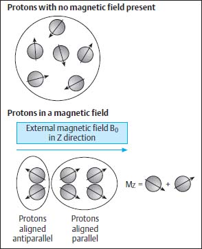
Fig. 1.1 Protons in a magnetic field
Top: In the absence of a magnetic field the magnetic moments of the protons are aligned statistically and their effects neutralize each other.
Bottom: Within the magnetic field Bo the majority of the protons are aligned parallel to the applied field while the minority are aligned antiparallel. The resulting longitudinal magnetization (MZ) of the tissue is the prerequisite for producing MR images.
Apart from setting up the longitudinal magnetization MZ, Bo also forces the protons into a precession movement around the Z-axis of the field, similar to a rotating spinning top precessing around the gravitational field of the earth. This rotation, or precession, frequency of the protons is also called the Larmor frequency ωo and is proportional to the strength of the magnetic field (Fig. 1.1).
ωo = γ × Bo
γ = gyromagnetic ratio = 42 MHz per tesla for protons
Excitation
MR systems have special receiver coils for picking up the signal sent back by the protons from the human body. These signals represent the raw data for reconstructing the MR image. The receiver coils of MR systems are oriented transversely to Bo in the XY plane, which explains why the longitudinal magnetization MZ does not induce a signal.
In order to measure a signal, MZ must be rotated into the transverse direction (XY plane). A magnetization that points in the transverse direction is referred to as the transverse magnetization or MXY. The rotation of M into the transverse plane (M becomes MXY) is called excitation. This is brought about by a radio-frequency pulse (RF pulse) that is sent by the transmitter coil at the appropriate frequency ωo (= Larmor frequency).
After excitation the protons are in the excited state. The magnetization has been flipped by 90° out of the Z direction into the XY plane (90° excitation) and rotates at the Larmor frequency ωo. The longitudinal magnetization MZ no longer exists (MZ = 0); it has become the transverse magnetization MXY. MXY now induces a voltage, the MR signal, whose strength is proportional to the magnitude of MXY.
Directly after excitation, the process of relaxation begins in which the protons leave the excited state and return to their state of equilibrium.
Relaxation
There are two relaxation mechanisms that describe the transition from excitation back to the equilibrium state:
 Longitudinal Relaxation Time T1
During longitudinal relaxation, longitudinal magnetization MZ recovers. Once longitudinal relaxation ends, the total magnetization is once again parallel to the applied field, the protons are in the state of equilibrium and the longitudinal magnetization MZ has regained its initial value prior to excitation (MZ = 100 %).
T1 time describes the rate at which the protons return from the excited state to the state of equilibrium.
The T1 relaxation times of tissues differ from each other:
• in tissues with a long T1 time relaxation occurs slowly,
• in tissues with a short T1 time relaxation occurs rapidly.
The associated relaxation process is called longitudinal relaxation, or T1, because the protons “relax” from the excited state back into the longitudinal direction of the magnetic field. Another term for T1 relaxation is spin-lattice relaxation because the energy absorbed by the protons (spins) during excitation is released to the surrounding tissue (lattice) during relaxation (Fig. 1.2).
 Transverse Relaxation Time T2
The signal that the transverse magnetization MXY induces after excitation is referred to as FID (free induction decay). The FID signal is high immediately after excitation and then becomes rapidly smaller as time progresses.
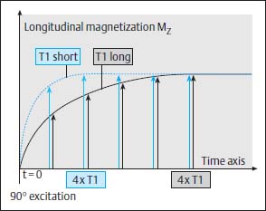
Fig. 1.2 Relaxation. Immediately after excitation MZ = 0 because the 90° excitation pulse has rotated the total longitudinal magnetization from the Z direction into the XY plane. After excitation MZ recovers with increasing time. Tissues with a short T1 time relax more rapidly than tissues with a long T1 time. The increase in MZ follows an exponential function. After approximately four times the T1 time of the tissue, T1 relaxation has finished, and MZ has reached its initial state before excitation (100 % MZ). During T1 relaxation the energy that the protons have absorbed during excitation is released back to the tissue as heat.
How Does this Signal Decay Occur?
Immediately after excitation all the protons precess in phase and their magnetic moments add up to form a large MXY and thus a large summation signal. Afterwards the protons are disturbed in their precession by their neighbors (i.e., other protons and molecules). Thus dephasing occurs, MXY becomes smaller, and the summation signal declines.
How are the Protons Disturbed?
Each proton as well as each molecule has magnetic properties that locally alter the main external magnetic field Bo of the magnet in their immediate vicinity. These tissue-specific effects are variable both in their size and over time. They depend:
• on the chemical binding state,
• on the electrical and magnetic properties of the tissue.
If only a single proton is observed, the effects that its neighbors exert are so complex that it is impossible to quantify them. With a whole host of protons as in the human body, however, the effects on one proton obey statistical laws and the net behavior of the protons becomes predictable, appearing in a temporal relationship to the transverse magnetization MXY.
Because the precession frequency of the protons is related to the strength of the local magnetic field, the field variations produced by the adjacent atoms influence the precession frequency in an unpredictable way. The protons precess somewhat faster or more slowly, depending on whether the main external field chances to be intensified or weakened by the tissue-specific effects. This results in divergence, the protons dephase, MXY and the signal become smaller (Fig. 1.3).
The dephasing of the protons after excitation is a relaxation process. The rate at which the protons dephase is characterized by the time T2.
The T2 relaxation times of tissues differ from each other:
• in tissues with a long T2 time, relaxation occurs slowly,
• in tissues with a short T2 time, relaxation occurs rapidly.
T2 time and signal decay are directly proportional:
• A long T2 time means that the protons affect each other only slightly, resulting in slow dephasing and hence slow decay of the signal.
• A short T2 time means that the protons affect each other strongly, resulting in rapid dephasing and thus rapid decay of the signal.
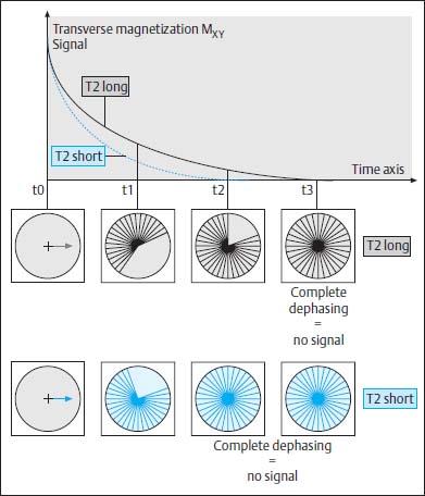
Fig. 1.3 Dephasing. Tissue-specific effects on the precession frequency of the individual protons cause dephasing. Dephasing can be visualized as a fanning out of the proton population. This fanning out causes the protons to “look” in different directions and their magnetic moments no longer sum up. This results in a reduction of MXY and signal loss. Tissues with a short T2 time lose their signal more rapidly because their relaxation is faster than in tissues with a long T2 time.
The Effects of Inhomogeneities
All the observations made so far with respect to transverse relaxation and the T2 time of the tissues are only valid when the magnet induces an ideal homogeneous magnetic field Bo, so that only tissue-specific effects can produce T2 relaxation and external disturbances are irrelevant.
What is a Homogeneous Magnetic Field?
An ideal homogeneous magnetic field is achieved when there are no fluctuations from the ideal field strength within the measurement range. Modern magnets do indeed reach a very high degree of homogeneity, but full 100 % homogeneity is not achieved. Apart from that, the patient’s presence disturbs the homogeneity.
What Effects do Inhomogeneities Have?
Because inhomogeneities are no more than fluctuations of the magnetic field, they result in different precession frequencies of the protons. This difference in precession frequencies causes an additional dephasing of the protons, which is superimposed over the tissue-dependent dephasing (T2 relaxation).
This is why in a real magnetic field with inhomogeneities the FID (free induction decay) decreases more rapidly than in an imaginary, completely homogeneous field.
The time constant T2, which is calculated in the real magnetic field with the aid of the FID, is therefore referred to as time constant T2*. The * indicates that this is a time constant that does not reflect the true tissue parameter T2, but rather that a second dephasing process is superimposed, which is dependent upon the quality of the field. The inhomogeneities cause the protons to dephase more rapidly. Therefore T2* is usually significantly shorter than T2.
How Can the Effects of Inhomogeneities Be Avoided?
Because the inhomogeneities of the external field are temporally constant, it is possible to compensate for their effect. With the aid of a second RF pulse (after the 90° excitation pulse), the 180° rephasing pulse, a signal is generated whose amplitude is not influenced by the inhomogeneities. This signal is called a spin echo (SE). Acquisition sequences using a 90–180° pulse sequence to generate an image whose signals are independent of inhomogeneities are referred to as SE sequences. Sequences without the 180° rephasing pulse are called gradient echo (GRE) sequences, the analogous signal being the gradient echo (GRE).
The 180° rephasing pulse compensates exclusively for the temporally constant inhomogeneities of the external magnetic field. However, the tissue-specific dephasing processes that result in T2 relaxation are not influenced. The intensity of the echo signal after a 180° rephasing pulse is therefore entirely dependent upon the tissue-specific T2 effects.
Various Image Contrasts
T1 contrast (T1-weighted image). Here image contrasts result primarily from the T1 differences of the tissues. The effects of T2 and proton density (PD influences) are minimized (yet still exist).
T2 contrast (T2-weighted image). In a T2-weighted image, contrasts result primarily from the T2 differences of the tissues. The effects of T1 and PD influences are minimized (yet still exist).
PD contrast (PD-weighted image). In a PD-weighted image, contrasts result primarily from the PD differences of the tissues. The effects of T1 and T2 are minimized (yet still exist).
T1-Weighted Image
 Repetition Time TR
The acquisition of only one echo is not enough for the entire raw-data set of one MR image because it contains too little spatial information to reconstruct the image. An echo signal forms only one line in the raw-data set.
The size of the raw-data set depends on the acquisition matrix of the MR image. For a matrix size of 256 × 256 pixels, 256 raw-data lines must be read in.
For the acquisition of each raw-data line, the slice usually has to be excited again. The time between two excitations is the repetition time TR.
One slice package containing several slices (multislice scan) can be acquired during the time TR, with the number of slices depending on the time TR.
 TR Time and T1 Contrast
The T1 contrast of an MR image is regulated with the aid of the TR time.
What Happens When TR Time is Long (TR >2500 ms)?
TR time can be selected so long that the net magnetization returns to its original position parallel to the magnetic field between the excitations. This is the case when TR time is set at four times as long as the T1 time of the tissue. In this case the protons have enough time for more or less complete T1 relaxation, and the state of equilibrium (= 100 % MZ) is always reached before the next excitation.
Because TR time is so long that T1 relaxation between two excitations is fully concluded in all tissues, there are no T1 contrasts visible on the image. (The image shows PD contrast; see p. 10.)
What Happens When TR Time is Short (TR = 400–800 ms)?
For a more understandable presentation, four time points will be considered (Fig. 1.4):
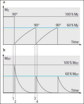
Fig. 1.4a,b Course of MZ and its effect on the signal.
The upper part of the illustration shows the Z magnetization and the course of T1 relaxation. The lower part of the illustration shows the transverse magnetization MXY and the signal and course of T2 relaxation. The time points 1–4 are explained in the text.
Time 1. Immediately before the first 90° excitation there is a state of equilibrium.
MZ1 = 100 %
MXY1= 0
Time 2. Immediately after the first 90° excitation: the excitation causes the magnetization to flip out of the Z direction into the XY plane.
MZ2 = 0
MXY2= 100 %
With increasing time MZ is set up again as a result of T1 relaxation.
Time 3. Immediately before the next 90° excitation: TR time is so short that MZ cannot be set up 100 %. At this point of time MZ3 is generated only by those protons that have relaxed during the (short) TR interval.
MZ3 <100 % (in this example 60 %)
MXY3= 0 (due to the rapid T2 relaxation)
Time 4. Immediately after the next 90° excitation: The 90° excitation pulse flips only the Z magnetization into the XY plane, which was set up in Z direction as MZ during the previous TR interval.
MXY4 = MZ3 (= 60 % in this example).
The result is a reduced signal on the MR image.
Saturation. Incomplete T1 relaxation during a short TR interval results in signal reduction on the MR image. This process is referred to as saturation. During a short TR interval the brightness of the tissues is determined largely by their T1 time:
• tissues with a long T1 time appear dark because they are more highly saturated,
• tissues with a short T1 time appear brighter because they are less saturated.
What Happens When TR Time is Very Short (TR = < 300 ms)?
If the TR interval is continually shortened, the saturation of all the tissues increases. Consequently they become hypointense and appear with little contrast.
Which TR Time for a T1-Weighted Image?
A TR time of 400–800ms has proven itself for the acquisition of T1-weighted images (Fig. 1.5).
 Contrasts of a T1-Weighted Image
The brightness of the tissues depends on their T1 time and thus on their saturation:
• water with the longest T1 time appears very dark,
• brain gray matter has a longerT1 time than white brain substance and is darker than the latter,
• fat has the shortest T1 time and is very bright.
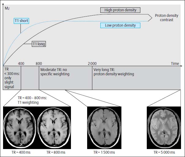
Fig. 1.5 TR time and T1 contrast. Because of the different T1 times of the tissues, T1 contrasts can be generated on MR images when the T1 relaxation of the tissues has elapsed to varying degrees within the TR time. With a TR time of 400–800 ms the T1 relaxation in tissues with a short T1 time has elapsed further than in tissues with a long T1 time, and the 90° excitation pulse flips (in tissues with a short T1 time) a larger magnetization (than in tissues with a longer T1 time). Therefore the signal of tissues with a short T1 time is larger than the signal of tissues with a long T1 time. The images demonstrate a strong T1 contrast. If the TR time is prolonged, contrast becomes less because the longitudinal magnetization MZ of all the tissues returns to 100%. With a very long TR time the contrast is PD contrast.
T2-Weighted Image
The T2 contrast of an MR image is regulated with the aid of the echo time TE.
 Echo Time TE
TE is the time between the excitation pulse and the recording of the echo signal.
If the signal is recorded at the echo time point then dephasing in the tissues, and thus also the signal, varies in strength (depending on the T2 time).
The signal differences measured are a reflection of the T2 effect:
• If the echo time TE is short, then the protons have little time to dephase and the T2 effect on the image is small.
• With a long TE echo time the protons have enough time to dephase and the T2 effect on the image is large.
 TE Time and T2 Contrast
What Happens When TE Time is Short (TE < 30 ms)?
Dephasing has advanced only slightly by the time the echo is acquired; the protons of all tissues are still precessing almost in phase. Because of the small amount of dephasing, MXY is large and all tissues appear hyperintense.
Low T2 contrast shows that MXY of all the tissues is still almost the same because no differences in the dephasing of the tissues have as yet developed during the short echo time.
What Happens When TE Time is Longer (TE = 70–150 ms)?
The tissue-specific effects are allowed to act on the protons for a longer time so that dephasing of all the tissues has advanced further. In comparison with an image with a short echo time TE, the signal from all the tissues has become smaller due to the increased amount of dephasing. In tissues with a short T2 time, however, dephasing has progressed further than in tissues with a long T2 time.
The tissues on the image appear with varying intensity:
• tissues with a short T2 time appear dark because dephasing has progressed further,
• tissues with a long T2 time appear bright because dephasing has progressed less.
Contrasts are a qualitative reflection of the T2 times of the tissues. Such an image is referred to as T2-weighted.
What Happens When TE Time is Very Long (TE >200 ms)?
Dephasing has progressed even further; all the tissues have lost even more signal.
Tissues with short T2 times are no longer displayed. Because the protons are completely dephased, MXY = 0 and can no longer induce any signal.
Tissues with moderate T2 times are hypointense due to the relatively large amount of dephasing of the protons.
Only tissues with very long T2 times, e.g., fluids, still appear bright due to the small amount of dephasing.
A very strong T2 contrast is visible on the image. The echo time however is too long to display tissues with short and moderate T2 times.
Which TE Time for a T2-Weighted Image?
For good T2-weighting a TE time of approximately 70–150 ms is appropriate in the majority of scans because with this TE time T2 contrasts are very good without too much loss of image signal (Fig. 1.6).
 Contrasts of a T2-Weighted Image
The brightness of the tissues depends on their T2 time and thus on their dephasing at the echo time point.
Related posts:
Stay updated, free articles. Join our Telegram channel

Full access? Get Clinical Tree


