Fig. 2.1
Basic OCT setup, with a beam splitter (BS) separating the light into the sample arm towards the tissue, and the reference arm towards the mirror, respectively. The plots display the source spectrum as well as the resulting interference pattern, and illustrate the reconstruction process. The tomogram t(z) broadens the discrete reflections in the reflection profile f(z) to a full width at half maximum (fwhm) characteristic of the OCT system
(2.1)
(2.2)
P dc in Eq. 2.1 corresponds to the light reflected individually from the reference and the sample arm. Of interest for OCT are the two interference signals in P ac.
Optical Frequency Domain Imaging (OFDI) [1] and other swept source implementations of OCT use a wavelength-swept laser source that sweeps a broad wavelength range in a short time. As a result, the interference signal recorded as a function of time corresponds to the signal as a function of the wavenumber k = 2π/λ. The first interference term of Eq. 2.1 can then be expressed as
Here, α(k) is the spectral shape of the source spectrum, and f(z) is the reflectivity profile. For a single reflector at depth z, the signal varies periodically as a function of the wavenumber. The rate of this variation increases linearly with z.
(2.3)
The integral of Eq. 2.3 can be identified as the Fourier transformation of the depth profile of the sample reflectivity. Recording the signal as a function of the wavenumber is equivalent to taking the Fourier transform of the axial reflectivity profile. Accordingly, inverse Fourier transformation of the recorded signal will reconstruct the tomogram t(z) of the sample reflectivity profile:
The Fourier transformation connects the spatial domain (z) with the spatial frequency or wavenumber domain k. This transformation is a standard operation and can be performed numerically with very high efficiency using the Fast Fourier Transform (FFT). The reconstructed amplitude |t(z)| is proportional to the amplitude of the electromagnetic field scattered from the sample at the same depth. Generally, one is interested in the squared norm T(z) = |t(z)|2, which is proportional to the intensity scattered from the sample as a function of depth. Because of the large dynamic range covered by the OCT signal, tomograms are displayed in logarithmic scale:

The fringe signal P ac contains two interference terms with mirror symmetry. If the first term results in a tomogram t(z), then the second term produces a tomogram t(−z), mirrored about the zero differential path length, as illustrated in Fig. 2.1. Generally, this results in a disturbing overlap that can be avoided by adjusting sufficient path length difference between the reference and the sample arm, or by employing additional strategies to separate the two terms.
(2.4)
(2.5)
Although the reconstructed tomogram is a close image of the original structure, the spectral shape of the source effectively performs a weighting of the spatial frequency spectrum. Only the range of spatial frequencies covered by the employed light source is accessible. As a result, the reconstructed signal is a filtered image of the original structure, expressed by the convolution of the original reflectivity profile with the point spread function (PSF) of the OCT system. This PSF is equivalent to the inverse Fourier transform of the spectral shape function a(z) = FT−1{α(k)}. The tomogram t(z) can be expressed as
with the star symbol indicating the convolution operator. a(z) is the coherence function of a light source with the power spectral density α(k), explaining the origin of the term ‘optical coherence tomography’.
(2.6)
As illustrated in Fig. 2.1, a single reflector in the original sample reflectivity function results in a peak of a finite width in the reconstructed tomogram. Assuming a source spectrum with a Gaussian shape, the full width at half maximum (fwhm) of the spectrum as a function of wavenumber is related to the fwhm of the peak in the reconstructed tomogram by
The wider the spectrum covered by the light source, the better the structure of the axial tomogram is resolved. Indeed, the axial resolution scales with 1/Δλ and the square of the central wavelength λc 2. Although the central wavelength of the source should be minimized to increase axial resolution, tissue absorption and scattering are increased at shorter wavelengths and diminish imaging penetration depth, as discussed in more detail in Sect. 2.4.2. Most OCT sources for intravascular imaging operate at a center wavelength close to 1,300 nm and have spectral widths of ~100 nm fwhm, providing an axial resolution below 10 μm.
(2.7)
Real OCT sources do not produce Gaussian spectral shapes, but aim at providing a very broad spectrum with a smooth shape. Because of the Fourier relation between the spectral shape and the PSF of OCT, any ripples or spikes in the spectrum would severely degrade the resulting tomogram.
2.2.2 Imaging Lateral Structure
In order to resolve structure in the lateral direction, the probe beam is focused into a small spot. It is then scanned in the lateral direction while constantly acquiring A-lines. At each scan location, the axial depth profile is acquired by one wavelength-sweep of the light source, resulting in one A-line. Assembling all A-lines of a lateral scan into a B-scan results in a cross-sectional image. The collection of multiple B-scans while scanning along the remaining spatial coordinate represents a three dimensional tomogram and is sometimes referred to as C-scan.
For intravascular imaging and probe-based imaging of other luminal organs, the natural way to scan a spot over the cylindrical inner surface of the organ is by rotating a side-looking imaging probe in the center of the lumen, as illustrated in Fig. 2.2. In a similar way, the collection of A-lines recorded during one rotational scan can then be assembled into the cross-sectional view of the vessel. In combination with a pull-back of the imaging probe, a helical scan pattern over the lumen surface is finally obtained, recording a full three-dimensional image of the organ.
Fig. 2.2
Principle of helical beam scanning and volumetric scanning
The shape of the laser spot on the tissue determines the lateral resolution of the imaging instrument. Light emitted from a laser source is characterized by its high spatial coherence, resulting in well-defined wavefronts, whose propagation can be accurately modeled with the Gaussian beam formalism, summarized in Fig. 2.3. A Gaussian beam is characterized by a Gaussian-shaped amplitude and intensity distribution in the lateral direction, with w designating the beam radius at the point where the field amplitude has diminished to e −1 of the peak value and accordingly the intensity has dropped to e −2, where e is Euler’s number. The minimum radius or waist, at the focus, is designated w 0. The collapse of a beam approaching a focus is mirrored symmetrically by expansion of the diameter (diffraction) as the beam propagates beyond the focus. The smaller the focal spot diameter, the more rapid the collapse and expansion. At a distance z 0 = (1/2)kw 0 2, the waist has increased by a factor sqrt(2). The Rayleigh-range of length 2z 0, centered on the focal plane is used to define the depth of field (DOF). Structure within the DOF is imaged with a lateral definition of within a factor of sqrt(2) of that at the focal plane. Sample regions outside the DOF are considered out of focus, and suffer from dramatically reduced lateral resolution and signal amplitude. If the DOF is matched to the typical image penetration depth of OCT within coronary tissue (~2 mm), then the lateral resolution is limited to approximately 20 μm.
Fig. 2.3
Principle of Gaussian beam propagation
A key feature of OCT is the decoupling of axial and lateral resolution. Whereas the source characteristics determine the axial resolution, the lateral resolution is defined through the focusing optics. The DOF and the lateral focus are directly coupled, however, and impose a limit on the lateral focusing.
2.3 Instrumentation
2.3.1 Interferometer
The ability to couple a coherent laser beam into a glass fiber and propagate the light within this fiber with only minimal loss has enabled modern telecommunication technology and facilitated many other applications involving laser light.
A single mode fiber consists in a thin glass core of 5–10 μm diameter, embedded in a slightly lower refractive index glass cladding. Although it is made of glass, the very small diameter of this structure ensures that the fiber remains flexible on the scale of centimeters and can be conveniently manipulated and configured.
The refractive index difference between the core and the cladding confines the light close to the core, similar to total internal reflection. Because the diameter of the core is so small, it accepts only a single spatial mode. This ensures that the light propagating along the fiber remains coherent and the beam emerging from the fiber is identical to the beam that was coupled into the fiber. The spatial shape of this mode can be approximated by a Gaussian mode. At the fiber facet, this mode exits the fiber and emerges as focused Gaussian spot that will inevitably diffract according to Gaussian beam propagation. Within the fiber, however, this intensity profile propagates unaltered, confined by the fiber structure.
Unlike free space components, fiber optics do not have to be aligned as the light is inherently guided within the fiber, and make robust and rugged optical systems. Catheter-based imaging probes are only possible due to the flexibility of optical fibers and offer the ability to relay an optical signal to and from the coronary arteries.
Figure 2.4 displays the schematic of a fiber-based intravascular OCT system [2]. The fiber carrying the source light is divided into two fibers, creating the sample and reference paths. Both signals are then fed through a fiber circulator. These non-reciprocal elements enable to efficiently relay the signals to the sample and the reference mirror, and the signals reflected from there to the detector. Unlike the double pass through the beam splitter of the free-space configuration, which directs half of the reflected signal back towards the light source, the circulators prevent this signal loss and provide an inherent signal advantage.
Fig. 2.4
Schematic layout of fiber-based interferometer for catheter-based imaging. RJ Rotary Junction, BS Beam Splitter, PBS Polarizing Beam Splitter, PC Polarization controller, LP Linear Polarizer, BR Balanced Receiver, A/D Analog to Digital converter
The optical path length of the sample and the reference arm must match precisely. Accordingly, the reference arm consists of several meters of fiber to compensate the catheter length of the sample arm. The reference mirror is mounted on a translation stage to enable rapid and easy adjustment of the precise path length.
At the detector, the sample field is combined with the reference field to interfere, by means of a fiber coupler or free-space beam splitter. In the Mach-Zehnder configuration displayed in Fig. 2.4, both outputs of the beam splitter feature an interference signal. Due to the law of energy conversation, the intensity of the two output signals together equal the intensity of the two input signals. Accordingly, a sample reflection that interferes constructively in one exit port features destructive interference in the other port. Mathematically, the sign of the interference terms in Eq. 2.1 is inverted between the two outputs. This opens the possibility of balanced detection: Detecting independently both interference signals, but digitizing only their difference effectively eliminates the P dc of Eq. 2.1 and conserves only the interference terms of interest. This approach also removes amplitude noise that is common to both channels. The reference signal frequently exceeds the sample signal by orders of magnitude and makes this detection scheme attractive by using the entire available dynamic range of the electronics for the interference signal.
It is important to consider that electromagnetic waves are vector waves and their oscillations are beating in a spatial direction. In the realm of paraxial optics, which is well suited to describe OCT and only excludes very tightly focused beams, the field oscillations are orthogonal to the direction of the beam propagation. If the vibrations are confined to a single direction along the entire propagating beam, the light is said to be linearly polarized. In general, a field oscillates in an elliptical fashion and can be described as the superposition of a beam with linear polarization along the horizontal direction and an identical beam, but polarized in the vertical direction and with a specific delay with respect to the horizontally polarized beam:
![$$ \overrightarrow{U}(z)=\left[\begin{array}{c}{U}^h(z)\\ {}{U}^v(z)\end{array}\right]=\left[\begin{array}{c} cos\ \gamma \\ {} sin\ \gamma {e}^{i\delta}\end{array}\right]U(z) $$](/wp-content/uploads/2016/09/A320873_1_En_2_Chapter_Equ8.gif)
γ determines the ratio between the two orthogonal polarization states, and δ defines the phase offset. Equation 2.7 describes the “Jones vector” of the field U. At the detector, only the part of the sample field that is polarized identical to the reference field will interfere with that reference signal. Writing the interference term for vector fields gives
where the dagger denotes the complex transpose. The sample field can be decomposed into a component parallel to the reference field, and a component orthogonal to it. The product with this latter cancels out and does not contribute to the interference signal.
(2.8)
(2.9)
Although its spatial profile is confined, the polarization state of light generally alters upon propagation along a single mode fiber. Indeed, this phenomenon is quite sensitive to bending and pressure applied to the fiber. A controlled amount of bending and twisting enables effectively to control and align the polarization state of the reference signal. In the practical case of catheter-based imaging, however, the sample fiber is manipulated and moved during the acquisition, and it is impossible to control the polarization state of the sample light. Further, the imaged tissue might exhibit birefringence and specifically alter the polarization state of the propagating probe beam.
To overcome the inability to control the polarization state of the sample light and avoid artifacts in the tomogram due to changes in the polarization state of the sample light, polarization diverse detection, as displayed in Fig. 2.4, is needed. The combined reference and sample signal is projected along two orthogonal linear polarizations by means of polarizing beam splitters. The reference light is adjusted to be linearly polarized at 45° in front of the detector with polarization controllers and a linear polarizer. This ensures an equal splitting of the reference signal into both polarization channels. The unknown sample polarization state is split into the same polarization basis. Each part of the sample light is now polarized in parallel with the local reference signal and creates the desired interference signal:
Taking the sum of the tomograms of both polarization channels T tot(z) = T v(z) + T h(z) provides a signal that is invariant of the precise sample polarization and is robust with respect to movement of the sample fiber.
(2.10)
2.3.2 Light Source
The ideal OCT light source for intravascular imaging should provide a rapid sweep of wavelengths over a wide spectrum centered around 1,300 nm. The width of the spectrum together with the smoothness of the spectral shape will define the axial width of the OCT PSF.
Developments in source technology have enabled a dramatic increase in OCT imaging speed. Although A-lines rates in the MHz range have been demonstrated, the digitization of the resulting interference signal becomes challenging [3, 4]. Also, at constant source power, an increase of sweep speed translates directly to a reduced number of photons, and results in a decreased signal strength and depth of imaging penetration. Current commercial instruments operate at A-line rates around 100 kHz.
The working principle of all sources is a broadband gain medium combined with a wavelength-tunable filter, which selects a narrow wavelength range at each instant in time. There is a wide range of physical implementations, ranging from fiber-based sources consisting in a combination of fiber-optic elements, to fully integrated micro-electro-mechanical systems (MEMS). Most sources produce an output power between 20–60 mW, resulting typically in ~8–20 mW power incident on the tissue.
Besides the A-line rate and the output power, important characteristics of a source are its duty cycle, the sweep linearity, and the instantaneous line width. The duty cycle expresses how much dead time passes between consecutive scans and should be high to optimally use the bandwidth of the detection electronics. The ideal sweep varies the wavenumber linearly with time. Any deviation has to be compensated with either a non-uniform sampling clock or interpolation of the digitized signal. Both can become challenging for strong non-linearity.
At each instant in time, any source will generate a spectral line of finite width, rather than a pure monochromatic signal. In consequence, the interference pattern does not sample a single spatial frequency at each time, but a narrow peak with a finite width. The larger the path length difference between a sample feature and the reference arm, the faster the modulation of its wavenumber signal. Variations within the finite spectral width of the source wash out and result in a decreased signal amplitude in the reconstructed tomogram. Mathematically, the sample spatial frequency spectrum is convolved with the instantaneous spectral shape. After reconstruction of the tomogram, this convolution translates into multiplication with the Fourier transform of the finite line width in the spatial domain, which is illustrated in Fig. 2.5.
Fig. 2.5
Measurement of single reflector placed at various depths to assess the signal roll-off with depth. The roll-off curve is the Fourier transform of the instantaneous spectral line of the wavelength-swept laser source. Also note the non-uniformity in the noise floor
The best signal amplitude is obtained at zero path length difference. However, to separate the tomogram from its mirror term, an additional path length difference is frequently introduced. This works well for sources with a very low roll-off and a very narrow instantaneous line width. Alternatively, it is possible to place an acousto-optic modulator in the reference arm [5]. Modulating the reference signal at a ¼ of the acquisition frequency has a similar effect as moving the reference arm by a distance equivalent to ¼ of the entire imaged depth range. Unlike a physical increase of the path difference, this reference arm modulation does not alter the spatial frequency spectrum and avoids a signal wash out. Instead, it axially shifts both the tomogram and the roll-off curve, and enables a separation of the two mirror terms, without trading off any sensitivity, as demonstrated in Fig. 2.5.
2.3.3 Catheter
The catheter is connected through the rotatory junction with the interferometer and relays the signal to and from the probe tip. It consists in a stationary narrow diameter (typically 0.87 mm) sheath that contains the rotating probe. The probe is fabricated from a single mode fiber and at its distal tip the light emerging from the core of the fiber is reflected to the side and focused through the transparent sheath material onto the lumen surface. The fiber does not tolerate rotational shear forces well and is embedded in a drive shaft. It consists of a coiled spring to preserve the flexibility of the catheter and transmit the torque from the rotary junction to the probe tip. This probe assembly can also be translated in the axial direction within the sheath to perform the required pull-back.
There are two types of distal optics to focus the fiber mode onto the lumen. One uses a ball lens design, and the other a graded index (GRIN) lens. The ball lens is fabricated by splicing a segment of pure, homogenous glass fiber (or “core-less” fiber) to the single mode fiber facet. The tip is then melted to create a drop-shaped glass ball by surface tension. Light emerging from the fiber core diffracts in the core-less medium and is refracted at the ball lens surface to converge into a focused spot. To obtain a side looking probe, the ball lens is angle polished to reflect the light by total internal reflection and to use the side of the glass-ball as the refracting surface.
Alternatively, a GRIN lens or GRIN fiber consists in a fiber-like element with a radially varying refractive index distribution. Propagation through this element is similar to propagation through a classical lens. Splicing an optimized sequence of core-less fiber, GRIN fiber and again core-less fiber at the facet of the probe fiber enables to generate the desired focal spot. Reflection to the side is achieved by a microprism, glued to the distal tip of the fiber optics.
Both probe types achieve focused spots having radii of 20–25 μm, and corresponding fwhm of the lateral PSF of 25–30 μm. However, the refraction of the beam at the curved sheath-tissue interface induces aberrations on the beam that can degrade its focusing and introduce an asymmetry between the direction along and transverse to the catheter axis. Interestingly, the imperfect shape of the ball lens in the lateral direction may be used to compensate for these aberrations. Ideally, the focus should be located just beneath the surface of the vessel lumen to match the depth-of-field to the available image penetration, and is targeted at ~1.5 mm from the sheath surface.
In order to suppress strong reflections from the sheath interface and guarantee total internal reflection in case of an angle polished reflector, the beam is usually reflected at an angle smaller than 90 deg. Accordingly, the resulting cross-sectional views correspond to conical cross-sections through the tissue volume.
Figure 2.6 displays schematics and photographs of two commercial catheters. The catheters have radio-opaque markers for visualization on the angiogram, and a provision for a thin (0.0014″) guide-wire for deployment.
Fig. 2.6
(a) Working principle of fiber-optic probes, for a ball-lens probe (top) and a graded index lens (bottom). Photographs of commercial catheters from Terumo (b) and St Jude Medical (c)
2.3.4 Rotary Junction
The rotary junction connects the interferometer with the catheter and defines the helical scan pattern of the optical probe. As schematically displayed in Fig. 2.7, it consists in a static collimation lens on the interferometer side, and a second lens on the catheter side that rotates together with the probe and couples the collimated beam back into a single-mode fiber. The alignment of these lenses is very sensitive and critical to avoid a strong rotational variation of the power coupled to the fiber probe. Physically, the proximal end of catheter is connected to this rotating fiber.