Physics of Ultrasound

Since its first ocular application (1) in 1956, ultrasound has had a broad impact on the practice of ophthalmology. It is now a standard clinical modality for measuring ocular dimensions, diagnosing and monitoring ocular diseases, and providing information regarding orbital diseases. Modern ultrasound systems provide real-time, highly detailed images of ocular structures in a rapid, noninvasive manner, posing no significant threat of tissue damage. Ultrasonic biometry quantifies ocular dimensions needed to plan and evaluate sight restoration and improvement by intraocular lens implants and corneal surgery. Real-time ultrasound images, unaffected by optical opacities, have significantly advanced the diagnosis and management of virtually all ocular diseases and abnormalities. Ultrasonic imaging of orbital disease and blood-flow patterns complements data obtained by other imaging modalities, such as magnetic resonance imaging (MRI).

The effective use of ophthalmic ultrasound requires a basic knowledge of its physical nature and the phenomena associated with its propagation and scattering. This understanding is important for proper interpretation of clinical results and avoidance of misleading artifacts that can arise in ocular examinations. It is also important for evaluating emerging techniques that promise to extend the scope of ultrasonic examinations in the future as well as to best use other techniques for complementary diagnostic value.

Ultrasound is an acoustic wave comprising compressions and rarefactions that propagate within fluid and solid substances (2, 3, 4). By definition, ultrasonic waves exhibit frequencies above 20 kHz,¹ and they differ from sound waves because these high frequencies render them inaudible. Because it is a wave, ultrasound can be directed, focused, and reflected according to the same general principles that govern these phenomena with other waves, such as light. The high frequencies (typically 10 MHz) and small wavelengths (e.g., 150 μm) available with ultrasound can provide the detailed resolution required for ocular examinations. Newer techniques use even higher frequencies (e.g., 50 MHz) to obtain wavelengths near 30 μm for very fine resolution within the anterior chamber (5,6).

Ultrasonic examinations of soft tissues use reflective (“pulse-echo”) systems analogous to those used in radar and sonar. This approach allows examination within a thin “slice” through tissue structures. A piezoelectric transducer serves as the ultrasonic transmitter and receiver. It generates a short burst of ultrasonic energy that propagates through the eye and undergoes partial reflection at tissue boundaries that exhibit abrupt changes in mechanical properties, including density and rigidity. These reflections, or echoes, return to the transducer where they are electronically detected. A-mode, or A-scan, systems graphically display these echoes as a function of time on a video monitor. B-mode systems generate cross-sectional gray-scale images (the gray scale corresponds to the A-scan amplitude) by scanning the transducer to address a series of lines through the eye; the amplitudes of received echoes control the brightness (or gray scale) along corresponding lines of a video image (B-scan). The terms A-scan and B-scan as well as C-scan and M-scan derive from early radar terms, using pulse position indicator (PPI) display.

Subsequent chapters describe how these A- and B-mode results are interpreted for diagnostic purposes. Proper interpretation requires an understanding of how A- and B-mode signals are related to underlying tissue properties and how they are affected by the characteristics of the ultrasonic system and transducer. The principles involved with ultrasonic imaging differ from those encountered with other imaging modalities. Computed
tomography (CT) measures the partial absorption of xradiation transmitted through the body, and MRI senses molecular phenomena elicited within tissue. Optical coherence tomography (OCT) senses light that is backscattered by local changes in optical refractive indices rather than mechanical properties (7). OCT can produce high-resolution cross-sectional images of ocular tissues, such as the retina, but, as with other optical techniques, its depth of penetration is limited by optically opaque media, such as the sclera and intravitreal substances.

The physical principles of ultrasonic imaging are reviewed in this chapter, which describes how ultrasound is generated and detected, how it is reflected and absorbed in tissue, and how various factors influence the resolution that can be achieved in examining the eye and orbit. (References 2, 3, 4 are comprehensive texts treating the physics of ultrasound.)

GENERATION AND DETECTION OF ULTRASOUND

The key element in any ultrasonic system is a piezoelectric transducer, which is used to generate an ultrasonic wave from an applied voltage signal and to detect ultrasonic echoes returning from within the eye. A typical transducer unit (Figure 1.1) consists of a thin disk of piezoelectric material, such as lead zirconate titanate (PZT), a backing section, and an acoustic lens, which focuses the generated ultrasonic beam. The entire unit is commonly referred to as the transducer, although this term applies most correctly to only the piezoelectric element; common usage is adopted in this text. In most clinical systems, the transducer is coated with a thin layer of coupling gel and held in contact with the globe or lid. The gel affords a transmission path for ultrasound, which is rapidly absorbed in air. Coupling can also be provided by fluid solutions confined in small chambers or surgical drape.

Generation and detection of ultrasound take place in the piezoelectric material. The molecular configuration of a simple piezoelectric crystal is shown schematically in Figure 1.2. The molecules exhibit net charge polarizations that are forced into alignment by the crystalline structure so that effective positive charge centers are oriented along the same direction. In the transmission mode, an ultrasonic pulse is generated by applying a voltage pulse across external electrodes plated on the crystal surfaces. The molecules tend to stretch or contract, depending on whether the voltage polarity causes attraction or repulsion of the charge centers. These molecular effects alter the overall crystal thickness in proportion to the amplitude of the applied voltage. When the polarity of the applied voltage is rapidly varied, the crystal executes corresponding rapid expansions and contractions, which constitute ultrasonic vibrations.

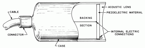Figure 1.1. Cutaway view of transducer.

In the receive mode, the crystal is compressed and expanded by an impinging ultrasonic echo pulse; the concomitant changes in molecular charge separation induce an output voltage whose amplitude and waveform depend upon the echo pulse. The voltage is readily measured as a function of time, enabling ultrasonic echoes to be detected as they return from the eye.

In the past, piezoelectric transducers were often fabricated from precisely oriented cuts of quartz crystals, which require large excitation voltages. Now, most transducers are fabricated from more sensitive materials, including lithium sulfate, ceramics (such as PZT), composite materials, and, for high frequencies, polyvinylidene fluoride (PVDF) membranes (8). Modern transducer materials can detect small ultrasonic signals, containing only microwatts of power. Some of these materials must be “poled” before they can be used in transducers. In this process, piezoelectric domains are brought into alignment by applying large, constant voltages at elevated temperatures. Once this alignment is achieved, these materials can generate and detect ultrasound in the manner described previously.

A piezoelectric transducer responds most actively to voltage signals and ultrasonic pulses that have frequencies near its resonant frequency. This frequency is determined by the material’s thickness, increasing as it is made thinner. Resonance effects can lead to prolonged series of ultrasonic vibrations, which are suppressed by using backing sections to achieve high resolution, as discussed in a subsequent section.

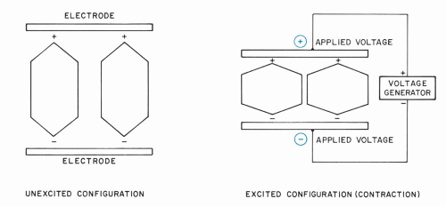Figure 1.2. Schematic representations of molecular configuration in a piezoelectric material illustrating contraction induced by an applied voltage.

PROPAGATION OF ULTRASOUND

When a piezoelectric transducer is immersed in a fluid and electrically excited, its thickness vibrations generate an ultrasonic wave of compression and rarefaction that propagates through the fluid. These waves, termed longitudinal or compressional ultrasonic waves, are the type used for tissue visualization. They propagate through soft tissues in the same manner as they propagate through fluids.

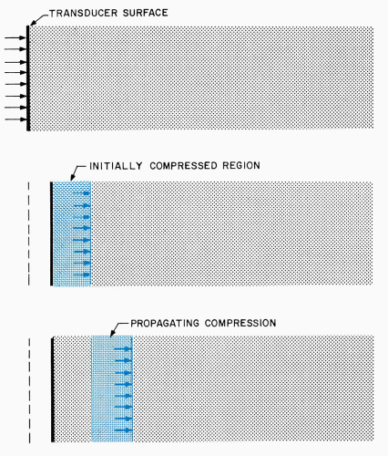Figure 1.3. Generation and propagation of a compressional ultrasonic wave. The wave is generated by a small extension of a transducer surface into a fluid.

Ultrasonic propagation is illustrated in Figure 1.3, where a voltage pulse causes a piezoelectric transducer
to undergo a small, rapid expansion. Extension of the front transducer surface initially compresses the adjacent fluid layer, elevating its density and pressure. Increased molecular collisions in this compressed region eventually couple the elevated density and pressure to the next fluid layer, while the initially compressed region returns to its original state. Thus, the compression passes from the first layer to a second region and, in the same manner, continually propagates to more distant regions in the fluid. Similar phenomena occur when the transducer contracts rather than expands. In this case, rarefaction characterized by lowered fluid pressure and density propagates away from the transducer.

Induced compression and rarefaction disturbances travel through a substance at a speed (velocity of propagation) that is determined by the density and compressibility of that substance. In materials with low compressibilities, such as metals, compression passes rapidly from layer to layer, and large propagation velocities are encountered (e.g., 6,000 m/sec). In contrast, materials that are more readily compressed, such as fluids and tissues, exhibit lower velocities (e.g., 1,524 m/sec in water). As shown in Table 1.1, ocular tissues exhibit propagation velocities close to those of water (9, 10, 11, 12, 13, 14, 15, 16, 17). The largest velocity is exhibited by the lens. Propagation velocities are temperature-dependent (18). Near 37°C, a 1°C-temperature rise typically increases velocities by about 1 to 2 m/sec, except in fat where an opposite trend occurs.

TABLE 1.1 Reported Mean Velocities of Ultrasound in Ocular Tissues

Tissue Accepted Velocity	Velocity (m/sec)	Temperature (°C)	Frequency (MHz)	Investigator (Reference)
Cornea 1,639 m/sec	1,632	22	4	Chivers⁹
	1,550	22	4	Oksala¹⁰
	1,553	22	10	Thijssen¹¹
	1,572	20	20	De Korte¹³
	1,575	37	60	Ye¹⁴
Sclera	1,744	22	4	Chivers⁹
	1,630	22	4	De Oksala¹⁰
	1,583	22	10	Thijssen¹¹
	1,597	20	20	Korte¹³
	1,622	37	60	Ye¹⁴
Vitreous 1,532 m/sec	1,508	22	4	Chivers⁹
	1,495	22	4	Oksala¹⁰
	1,532	37	4	Jannson¹²
	1,506	22	10	Thijssen¹¹
	1,514	20	20	De Korte¹³
Lens 1,641 m/sec	1,548	22	4	Chivers⁹
	1,650	22	4	Oksala¹⁰
	1,641	37	4	Jannson¹²
	1,620	22	10	Thijssen¹¹
	1,659	37	15	Coleman¹⁵
	1,590	20	20	De Korte¹³
Cataractous lens	1,629	37	—	Coleman¹⁵
Water	1,524	37	—	Willard¹⁶
Aqueous humor	1,532	37	—	Jannson¹²
Fat	1,476	24	—	Frucht¹⁷

In medical systems, brief excitation voltages are used, and the transducer surface vibrates back and forth several times at a rate equal to its resonant frequency (e.g., 10 MHz). This series of vibrations generates several contiguous regions of compression and rarefaction that propagate with the previously mentioned velocity, as shown in Figure 1.4. These regions travel together as an ultrasonic pulse and cause, roughly, sinusoidal variations in density and pressure as they traverse the eye. Clinical systems use only small transducer motions (total excursions under one micron), and imperceptible and innocuous pressure variations are produced within the eye and orbit.

Sinusoidal ultrasound pulses manifest a wavelength that is an important determinant of many operational parameters, including resolution. The wavelength, Λ, is the spatial distance over which the pressure perturbation undergoes one complete cycle. Wavelength is determined by the frequency, f, of transducer vibrations and the propagation velocity, c, of the medium:

Λ = c/f

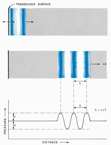Figure 1.4. Propagation of sinusoidal ultrasonic pulse in a fluid medium at two instants of time. Lower plot shows ultrasonic pressure variation of peak amplitude p. Static pressure level is exhibited outside the region occupied by the pulse.

This relation is obeyed because the transducer generates the same pressure level every 1/f seconds, and this pressure travels at a velocity equal to c. In water, 10-MHz operation produces a wavelength of 0.15 mm, which is commensurate with retinal thickness; increasing the frequency to 50 MHz decreases the wavelength to 0.03 mm, and thus increases resolution.

The wavelength describes the spatial distribution of pressure at a single instant of time. However, ultrasonic pulses continually propagate through tissue structures at high velocities, causing rapid pressure oscillations as they travel through points within the eye. In fact, as shown in Figure 1.5, the pressure at a point in the eye varies at the same high rate (e.g., 10 MHz) at which the transducer vibrates.

Nonlinear propagation effects, which distort ultrasonic pulses, can become significant at elevated ultrasonic pressure amplitudes (19). These effects occur because the acoustic propagation velocity is inversely proportional to density. Thus, the high pressure (high density) regions in Figure 1.4 actually travel at a somewhat slower speed than the low pressure (low density) regions of the pulse. The magnitude of this effect depends upon the nonlinearity property (“B/A” parameter) of tissue. As the pulse propagates, this speed differential acts in a cumulative manner and can distort the pulse by shortening
its compression regions and lengthening its rarefaction regions.

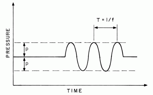Figure 1.5. Pressure variations caused as ultrasonic pulse passes through point A in Figure 1.4. The frequency of these variations is the same as that of the transducer vibrations.

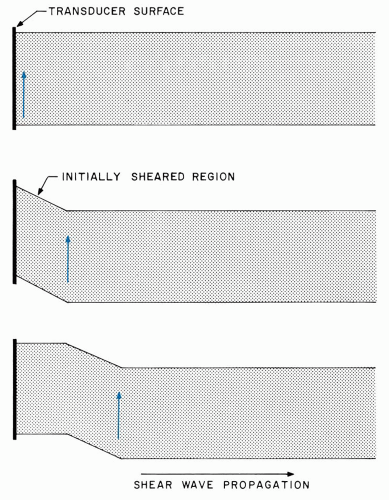Figure 1.6. Generation and propagation of shear ultrasonic wave in a solid. The wave is generated by a shearing force at the transducer surface. Internal displacements are perpendicular to direction of propagation.

Thus far, longitudinal, or compressional, ultrasonic waves have been discussed. Several other types of ultrasonic waves can be generated in certain materials but are not important in ophthalmic examinations. Surface (Rayleigh) waves and shear (transverse) waves are examples of these. Shear waves are excited in solids when a transducer surface vibrates within one plane (Figure 1.6). This motion generates shear forces that are transmitted to progressively farther regions within the solid; the induced particle motion is perpendicular to the propagation direction. Shear waves have not been used for ocular visualization because they do not couple well into tissue and because they are rapidly dissipated by viscosity.

REFLECTION AND SCATTERING OF ULTRASOUND

Ultrasonic pulses are reflected at boundaries between media that possess differing mechanical characteristics. Figure 1.7 illustrates the extreme case of total reflection from a rigid planar structure bounding a fluid of depth L. When the incident compression reaches the structure, the expansive forces accompanying molecular collisions are redirected back into the fluid, and the phenomena described previously cause the pulse to travel through the fluid in the reverse direction. The reflected pulse arrives back at the transducer after a time interval equal to 2 L/c, and it generates a corresponding output voltage, as shown in the figure. Observation of this voltage enables the boundary to be detected and permits L (distance) to be calculated if c (velocity) is known.

In the eye, a similar reflection arises whenever a pulse encounters a boundary between most ocular structures. However, ocular tissues exhibit similar mechanical properties so that only a small fraction of the incident pulse is reflected. Most of the incident energy is transmitted through the boundary, where it undergoes partial reflections at each successive interface.

The major reflective surfaces in the normal eye are those of the cornea, lens, and rear wall layers. Figure 1.8 shows a schematic diagram of these surfaces with typical dimensions and also illustrates the transducer echo voltages that arise from each of them. Corresponding clinical results are shown in Figure 1.9. This figure presents the radiofrequency (RF) echoes measured directly at the transducer as well as their envelopes, or video signals, that are used to modulate brightness or gray-scale levels in B-mode images.

The time interval between echo voltage pulses can be used to determine the thickness of the corresponding
tissue segment because the pertinent propagation velocities are known. Specifically, the time interval between successive echoes is equal to 2 L/c, where L is the corresponding tissue thickness. Thus, typical lens echoes are separated by 5 μsec (microsecond, which is 10⁻⁶ seconds; nanosecond [nsec] denotes 10⁻⁹ seconds) because L = 4 mm (a typical lens thickness) and c = 1,641 m/sec. Biometric systems using this approach have achieved a precision (reproducibility) of ± 20 μm in axial length determinations, and 40-MHz systems have achieved a precision of better than ± 2 μm in measuring the thickness of the corneal epithelium.

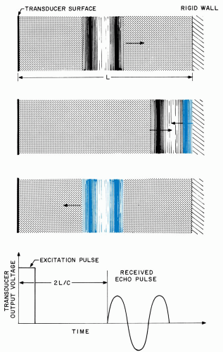Figure 1.7. Total reflection of an ultrasonic pulse from a rigid boundary. The transducer output voltage displays both the excitation pulse and the echo pulse so that the total transit time can be measured.

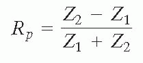
The amplitudes of ultrasonic reflections depend upon the characteristic acoustic impedances, Z, of adjacent tissues. The characteristic impedance of a tissue is equal to the product of its density, p, and propagation velocity:

Z = p c

The pressure reflection coefficient, R_p, is defined as the ratio of the reflected pressure amplitude to that of the incident pressure amplitude. For smooth tissue interfaces that are perpendicular to the ultrasound beam, R_p is equal to: