Olivier BEUF1, Philippe GARTEISER2, Kevin TSE VE KOON1 and Jonathan VAPPOU3 1 CREATIS, CNRS, Inserm, INSA Lyon, Université Claude Bernard Lyon 1, France 2 Centre de recherche sur l’inflammation, Inserm, Paris, France 3 ICUBE, CNRS, Université de Strasbourg, France Many pathologies affect the tissue structure and composition at different levels, including cellular modifications and the interactions between cells and their close surroundings, from the extracellular matrix up to the entire organ. Since the tissue structure and its composition determine how these tissues deform in response to an applied force, there is a correlation between the mechanical properties and the pathologic tissue alterations. Due to this fact, the measurement of mechanical tissue properties or “elastography” has been proposed as a quantitative marker of pathological or healthy conditions. Several development works have been dedicated to imaging methods that would be capable of measuring the mechanical properties in a clinical setting. Historically, ultrasound elastography was the first instance of virtual palpation. Magnetic resonance imaging was later adopted as an imaging tool to develop magnetic resonance elastography (MRE). Regardless of the underlying imaging method, all elastography approaches are based on three aspects: the application of a static or dynamic constraint, the measurement of the induced deformation and the reconstruction of mechanical properties. In the case of MRE, these elements consist of the generation and propagation of a shear wave, a phase-contrast MRI sequence and a quantitative reconstruction starting from the estimation of the shear modulus. Figure 7.1. Schematics of a pneumatic transducer employed in a clinical setting. The passive transducer is placed upon the thorax to transmit shear waves to the liver. Image from Resoundant (Rochester, MN, USA) Frequencies in the order of 50 Hz are typically used in clinics or even higher frequencies, in particular in preclinical scanners, where higher spatial resolutions are required. Several driver technologies are employed to produce shear waves in the region of interest. The most common approach in clinical settings is pneumatic excitation: a loudspeaker located outside the MRI room delivers acoustic vibration via a semi-rigid tube to a passive transducer made of a chamber with a membrane that vibrates in contact with the patient’s skin (Venkatesh et al. 2013), as illustrated in Figure 7.1. Mechanical excitation can also be generated by an electromechanical or piezoelectric transducer and can be transmitted as a rigid motion to the MRI room, delivered directly to the actuator (Tse et al. 2009) or obtained from the rotation of an axis with an eccentric mass at its end in contact with the patient (Runge et al. 2019). In such practical conditions, which are the most common ones, the displacement induced in tissues by the external transducer can be considered to be well represented by a harmonic plane shear wave. This hypothesis enables applying well-established wave propagation equations to estimate local mechanical properties. The equation of a propagating wave in a linear viscoelastic medium is given by: where ρ is the tissue density, ω is the angular frequency of the wave and u is the displacement field (and Δ is its Laplacian). Here, the mechanical properties are composed of a real part µ corresponding to the elasticity of the tissue and of an imaginary part ωη corresponding to its viscosity that together can be represented as a complex shear modulus G: The real part of G is the storage modulus, sometimes denoted as G′, and corresponds to the elasticity of the tissue, whereas the imaginary part, or loss modulus G″, is related to its viscosity. The magnitude of G and the damping ratio G″/2G′, derived from the representation of the complex value G in polar coordinates, are sometimes employed. In this way, we obtain the fundamental equation that relates the displacement induced by the wave to the mechanical properties of the medium in which it propagates: To visualize the waves generated via the different vibration devices mentioned above, motion-sensitive imaging sequences have to be used. For this purpose, encoding gradients are added to standard sequences such as gradient echo or spin echo sequences. The employed encoding gradients are designed to create a phase change in the signal that is proportional to the displacement (Lewa 1991). In order to solve equation [7.3], instantaneous tissue displacement has to be detected. This is achieved by temporally synchronizing the encoding gradients ( In practice, most often, gradients (typically with a sinusoidal or trapezoidal shape) that oscillate at the same frequency as the mechanical wave are used. Tissue displacement can also be described as sinusoidal motion whose frequency is imposed by the transducer and whose amplitude and phase vary within the sample. When required, the different spatial components of displacement can be estimated by consecutively encoding the motion with gradients oriented along the three spatial directions. Once the phase images are obtained, phase unwrapping followed by a conversion from radians to micrometers is performed to obtain the displacement field If we consider a (plane) shear wave that propagates in the y-direction with displacement motion along the z-direction, the displacement field can be expressed as: A represents the amplitude of this wave, ω is its frequency, k is the wave vector, oriented here along the y-direction, and θ0 is the initial phase of the wave which for now we consider equal to zero. Equation [7.4] shows that in order to encode this wave displacement into the phase of the MRI signal, the gradient where ?0(?) is a periodic function (often with the same period as the wave). Figures 7.2(A)–(C) illustrate the phase encoding in a relatively simple case of a plane wave generated by a vibrating plate with a frequency of 50 Hz and amplitude of 25 µm described by equation [7.5] and a trapezoidal gradient with the same frequency of 50 Hz and an amplitude of 40 mT/m. Figure 7.2(B) shows the displacement obtained at four separate points along the direction of propagation as well as the phase variation (according to equation [7.4]) when the motion encoding gradient is applied for one period. Figure 7.2(C) represents the final phase value depending on the position along the direction of propagation. As we can see, the phase provides an image of the displacement field. Other images at different instants of the wave propagation are required; this is achieved by repeating the acquisition with a delay between the motion and the application of the encoding gradient. Usually, at least four different sequential acquisitions are performed. By observing the obtained encoded phase in Figure 7.2(C), it can be noted that its absolute value is greater than π. In MRI, the signal’s phase is bounded between –π and π and this means that the acquired phase image will exhibit phase wraps, which can be easily unwrapped in the present example. However, phase continuity between the different acquisitions must be ensured as well, and in the case of more complex or noisy displacement fields, the phase unwrapping step can be quite difficult. Figure 7.2A. Schematics illustrating a device for generating shear waves within a phantom Figure 7.2B. Motion-encoding gradient (40 mT/m amplitude, 50 Hz frequency) as a function of time, wave (25 μm amplitude and 50 Hz frequency) and phase encoding obtained at four equidistant points along the propagation direction during one period Figure 7.2C. Phase accumulated after one period at different points along the di ection of propagation. However, the phase of the acquired MRI signal is affected by other physical phenomena that are static most of the time, that is, constant over time. The most common effect is related to the non-uniformities of the static magnetic field B0, which translates into a static phase ?s in the acquired images. In order to remove these undesirable effects in MRE, two acquisitions are performed with opposite polarities of the motion-encoding gradients, and the phas signal of interest is retrieved by subtracting the phase images of the two acquisitions. However, since phase images can exhibit different wraps that are not necessarily well localized, the phase related to the wave is typically extracted from complex images: Phase encoding by means of encoding gradients can be added to any kind of MRI sequence. Such gradients are executed after the excitation pulse and before the signal readout gradients, which, as a consequence, increases the echo time. Figure 7.3 represents the case of a gradient echo sequence where motion encoding is performed along the slice direction. Encoding the motion along the other directions is possible as well; displacement fields are commonly acquired in a sequential way along the three orthogonal spatial directions in advanced scans, or even along oblique directions by exploiting the simultaneous application of several gradient directions in order to maximize the effective gradient amplitude. The sequence chronogram in Figure 7.3 additionally shows that motion is triggered before the encoding gradients are applied, such that a stationary state of the shear wave is achieved. In some cases, motion is continuously induced, but this requires choosing a TR of the sequence equal to an integer number of motion periods and ensuring the absence of any time drift between the different clocks intervening in a scan (the MRI system clock and vibration device). The accumulation of small delays over several consecutive TRs yields an increasingly negative impact over the scan’s duration. In order to probe different instants of the wave propagation, a phase offset ? is introduced between the wave and the motion-encoding gradient. Four acquisitions (corresponding to four different values of ?) are usually performed with a constant phase offset over the interval [0, 2π[, referred to as different phase steps. The employed frequency of the shear wave is chosen depending on the targeted organ or tissue and on the achievable spatial resolution. Since the wave attenuation increases with increasing frequencies, it is important to choose an appropriate frequency that enables sufficient penetration into the investigated region. Thus, in most clinical MRI scans, the employed frequencies vary between 20 Hz and 200 Hz. The lower frequency boundary is related to the corresponding wavelength. Although a local wavelength measurement is sought (from which to extract the shear speed or shear modulus), it is necessary that the reconstruction step be performed with wavelengths shorter than the size of the targeted organ. Because of this, small-animal applications employ higher frequencies, varying from 200 Hz to approximately 1 kHz. Figure 7.3. Chronogram of a magnetic resonance elastography sequence based on a gradient echo sequence and an encoding gradient with a duration of three periods along the slice direction One last aspect to be taken into account is related to the acquisition matrix in the slice plane. The resulting image should provide a visualization of the wave propagating inside the region of interest, which defines the maximum pixel size in the image plane. On the other hand, the minimum size is imposed by the resulting SNR of the image. A general rule is to choose a pixel size such that a wavelength covers the equivalent of about ten pixels while ensuring an SNR greater than 10. Once the displacement field has been encoded into the phase of the MRI signal, the last step is the reconstruction of the mechanical properties. Overall, the various reconstruction methods can be classified into three categories: It is thus possible to determine the shear modulus µ by discretizing the above equation. This apparently simple method does however have the major disadvantage of being sensitive to noise. We shall see how some conditioning steps such as frequency filtering can significantly improve the robustness of this method. Before any inversion algorithm is applied, the first step is to unwrap the phase. The latter is obtained as the arctangent of the ratio between the imaginary part and the real part of the MRI signal, hence it is confined between -π and π. From a physical point of view, there is no reason for the phase to be restricted only to this range and an unwrapping step is often required to retrieve the actual phase. A second step that is widely employed in MRE, including in clinical MRE, is filtering based on the temporal Fourier transform (TFT). Applying the TFT is much more than a simple pre-processing step, since it leads to direct implications regarding the MRI scan: for example, the N phase steps required for the TFT (typically, N = 4) usually imply N different acquisitions and a scan time multiplied by the same factor. For each voxel of the region of interest, the TFT is applied to the N measurements, thereby selecting the displacement occurring at the frequency of mechanical excitation while filtering out the other frequency components. This step significantly improves the robustness of the reconstruction. The LFE method is rather complex and our goal here is to illustrate its main aspects. The reader can find detailed explanations in Manduca et al. (2003) as well as in the original article by Knutsson et al. (1994) about radar signals, which is the foundation for the LFE method in MRE. This method is based on processing steps following a spatial Fourier transform of the wave image. Clearly, spatial frequencies ν (and thus, indirectly, shear wavelengths λ from λ =1/ν) are located in the Fourier space, although without any information on their localization in space. The LFE method enables localizing the spatial frequencies of the Fourier domain in space. For this purpose, it can be shown that the local spatial frequency ν of a signal S can be found by applying lognormal filters Ri and Rj with central frequencies νi and νj, respectively: with ri and rj the inverse Fourier transforms of Ri and Rj, respectively. In summary, the LFE algorithm is composed of the following steps: Once these operations have been performed, a map of spatial frequencies ν(x,y) = 1/λ(x,y) is obtained, and hence the shear modulus µ(x,y) is retrieved with the hypothesis of a purely elastic and incompressible medium via µ = ρ.λ².f2, where f is the excitation frequency. Figure 7.4 represents the three steps required to perform an MRE acquisition. Figure 7.4. Illustration of the three steps of an MRE acquisition. (a) Generation and transmission of a shear wave in the region of interest, (b) visualization of the motion on the phase images of an MRE scan and (c) mapping of the mechanical properties by means of reconstruction algorithms. Data obtained in a gel made up of 2.5% gelatine with a stiffer inclusion (4% gelatine). The way to encode the MRE signal has evolved significantly since the first sequence was proposed (Muthupillai et al. 1995). Each modification has sought to perform faster scans, increase the amount of information acquired or decrease the echo time to increase the SNR. Some of such sequences are non-exhaustively described in this section. One of the characteristic MRE limitations is related to the duration of the motion-encoding gradients. Since they are applied after the excitation pulse of the imaging sequence, their duration leads to an increase in the echo time causing a loss of signal. This is further reinforced at lower mechanical frequencies. The goal of fractional encoding is to remove this undesired coupling between the applied mechanical frequency and the available signal at the price of reduced sensitivity to motion. The idea is based on the fact that, according to equation [7.4], it is possible to obtain a non-zero phase accumulation even when the gradient shape is different to the case illustrated in Figure 7.2(B). In practice, encoding gradients are executed with a frequency higher than the mechanical frequency. This enables a decreased echo time, thanks to the shorter duration of the motion-encoding gradients, and, hence, a gain in signal. Such a strategy can become advantageous in particular in organs such as the liver, where some pathologies are characterized by a strong loss of signal. On the other hand, the difference between the mechanical frequency and the encoding gradient frequency leads to a reduced accumulation of phase, all the more so as a smaller fraction of the mechanical vibration cycle is exploited for the encoding. The ratio q between the duration of the encoding ?G and the period of the mechanical oscillation T (or, equivalently, between the mechanical frequency and the encoding frequency),
7
Quantitative Biomechanical Imaging via Magnetic Resonance Elastography
7.1. Fundamentals of magnetic resonance elastography
7.1.1. Introduction

 in equation [7.4]) with the mechanical vibration and repeating the measurement for different phase offsets between the encoding gradient and the mechanical vibration. The obtained phase can be expressed in terms of the time profile of the gradients and the tissue displacement at a point
  in the image:
 . The compression displacement component is then removed (using one of the several available methods) to obtain the complete shear displacement field (typically as amplitude and phase data in the acquired image domain). The latter is then used to perform a local inversion of equation [7.3], thus leading to an estimation of G over the entire image or on an area of the image where both wave propagation and sufficient signal-to-noise ratio (SNR) are obtained.
7.1.2. MRE signal encoding
 has to have at least one component parallel to the direction of tissue displacement (z in equation [7.5]). Ideally, to maximize the encoding,
  is chosen such that:


7.1.3. MRE data reconstruction
7.1.3.1. Fundamentals

7.1.3.2. Pre-processing/conditioning
7.1.3.3. LFE method: local frequency estimation


7.2. MRE sequences
7.2.1. Fractional encoding
 , then represents a characteristic variable in the sequence. By integrating equation [7.4], in which the gradient shape is replaced by a sinusoidal signal with a pulsation ?G (period ?G) and an amplitude ?MEG, the accumulated phase ϕ over a given encoding duration ?G is expressed with respect to the ratio q as:


Related posts:

Stay updated, free articles. Join our Telegram channel

Full access? Get Clinical Tree


