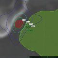
Radiobiology of High Dose Fractions

Fig. 5.1

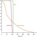
The solid line shows the typical variation of cell survival with fraction size as predicted by the standard linear-quadratic (LQ) model [Eq. 5.2]. The curve is characterised by a finite initial slope at zero dose and an ever-increasing slope as dose increases. In practice however, most human cell lines do not bend downwards indefinitely but tend to a finite limiting slope (dotted line). In the case illustrated here the deviation in response from the standard LQ prediction begins at around 6–7 Gy and thereafter becomes increasingly significant, with the LQ model over-estimating the effect actually achieved. Radiobiological assessments of treatments which utilise high dose fractions (typically >10 Gy) must therefore make allowance for this potential weakness in the basic LQ model

Although the LQ model remains the method of choice for quantitative evaluation of radiotherapy treatments, it should be noted that the earlier multi-target (MT) model does predict the observed “straightening out” of cell survival curves at higher doses. In practice the MT model is much less amenable to clinical application than the LQ model (especially over the conventional range of dose/fraction) but, as discussed below, attempts have been made to empirically combine the main features of the two models in order to provide better predictions over a wider dose range.

5.2 The Basic LQ Model

The LQ model was originally used to provide an empirical fit to observations on radiation chromosome damage by Lea & Catcheside [9] and also to fit radiation induced suppression of broad bean growth and development by Gray and Scholes [10]. However, LQ-type formulations can also be developed from more rigorous bio-physical considerations by considering how radiation damage accrues from immediately lethal radiation events and from the complementary interaction of sub-lethal events irrespective of their precise molecular basis [1, 11, 12]. The propensity for lethal damage to be created through these two alternative processes is reflected in the two radiosensitivity coefficients (α[alpha] and β[beta]) which are principal features of the model.

The essential mathematics behind the LQ model is as follows:

For a single acute fractional dose of magnitude d, the total number of lethal lesions produced is L, where:

$\mathrm{L}=\alpha \left[\mathrm{alpha}\right]\mathrm{d}+\beta \left[\mathrm{beta}\right]{\mathrm{d}}^2$

(5.1)

The surviving fraction of cells (S) is expressed as the probability of no lethal hits as deduced from Poisson statistics and is written simply as:

$\mathrm{S}= \exp \left(-\mathrm{L}\right)$

$\mathrm{i}.\mathrm{e}.:\kern0.24em \mathrm{S}= \exp\;\left[-\alpha \left[\mathrm{alpha}\right]\mathrm{d}-\beta \left[\mathrm{beta}\right]{\mathrm{d}}^2\right]$

(5.2)

Equation 5.2 describes the shape of the LQ cell-survival curve for a specific cell line or tissue type in terms of the relevant α[alpha] and β[beta] values which characterise them and, as noted above, is characterised by a continuous downward curvature (ie increasing steepness) with increasing d. When plotting cell-survival curves it is the universal practice to use a linear scale for d (on the x-axis) and a logarithmic scale for S (on the y-axis). The adoption of this convention allows easy visualisation of the characteristics of cell survival curves and of any differences that may exist between alternative cell lines.

In Eq. 5.2 the magnitude of α relative to β[beta] determines the increment of effect with increasing dose per fraction, the trend becoming more particularly pronounced at higher fraction doses. This is because the β[beta]-component of cell kill is related to the square of the dose (d²) and it thus follows that the downward curvature of the cell survival curve will be more pronounced in tissues for which β is relatively large compared with α[alpha], i.e. in tissues with lower α[alpha]/β[beta] ratios. Since late-responding normal tissues (LRNTs) are usually associated with smaller α[alpha]/β[beta] values than are many fast- growing tumours (typically 2–5 Gy cf 7–20 Gy), it follows that the LQ cell-survival curves of the former will exhibit more pronounced curvature than the latter.

In practice the cell surviving fraction is a cumbersome measure of treatment efficacy and a more useful parameter to use is the so-called Biologically Effective Dose (BED). BED is a measure of the overall “biological impact” of a schedule and takes account of the specific radiation response characteristics of the irradiated tissue by means of the inclusion of the relevant α[alpha]/β[beta] value in its calculation. Thus, even though two adjacent tissues might each receive the same radiotherapy fractionation schedule, their BEDs can be different because of the different tissue specific α/β[beta] values. The usefulness of the BED concept lies in the fact that it allows the design of new schedules (which may involve different fractionation) to be iso-effective to existing, well-tried, schedules. Since there are two ways of matching iso-effectiveness (for the tumour and LRNT responses) then there is the possibility of designing a new schedule which is radiobiologically superior, i.e. in terms of increased tumour BED and/or reduced LRNT BED.

In words, BED is defined to be the negative of the logarithm of surviving fraction, divided by the linear radiosensitivity coefficient (α[alpha]). More usefully, BED may be thought of as the dose required if given in ultra-small fractions and represents the ‘ceiling’ dose capable of causing the observed effect. Derivation of the BED from Eq. 5.2 is thus effected by taking natural logarithms of both sides of the equation and dividing throughout by α[alpha]:

$BED=-\frac{ \ln S}{\alpha }=d+\frac{d^2}{\left(\alpha /\beta \right)}$

(5.3)

Equation 5.3 provides the BED value for a single fraction. For a complete treatment involving N well-spaced fractions the resultant BED (BED_N) is simply N times larger than the single fraction BED, i.e.:

$BE{D}_N=N\left(d+\frac{d^2}{\left(\alpha /\beta \right)}\right)$

(5.4)

Equation 5.4 is usually written in the more familiar form:

$BE{D}_N=Nd\left(1+\frac{d}{\left(\alpha /\beta \right)}\right)$

(5.5)

Since Nd is the total physical dose delivered in a treatment, it follows that the BED is the product of the physical dose and a factor [the bracketed term in Eq. 5.5] which is dependent of the dose/fraction and the α[alpha]/β[beta] value characteristic of the tissue under consideration. As noted earlier, LRNTs are generally characterised by smaller values of α[alpha]/β[beta] and therefore, for a given N and d, are associated with a higher BED than tumours. Once calculated, BED acts as a reference value for iso-effect so that it is possible to estimate the dose per fraction and number of fractions required to achieve the same BED using different schedules.

5.3 Example of Simple LQ Modelling

Suppose it is required to emulate the biological effects of a conventional (60 Gy in 2 Gy-fractions) treatment with a single fraction treatment involving highly-focussed beams. What single fraction dose should be delivered?

Firstly, we consider the tumour (assumed α[alpha]/β[beta] = 10 Gy for a rapidly growing tumour). From Eq. 5.5, the BED (BED30) delivered in the conventional 30-fraction treatment is:

$BED30=30\times 2\times \left(1+\frac{2}{10}\right)=72G{y}_{10}$

(5.6)

(The Gy suffix of 10 is simply a reminder of the α[alpha]/β[beta] value used in the calculation).

If X is the total dose required in the single-fraction treatment to deliver this same BED then, from re-application of Eq. 5.5 it follows that:

$1\times X\times \left(1+\frac{X}{10}\right)=72G{y}_{10}$

(5.7)

Equation 5.7 is a quadratic equation for which the solution is X = 22.3 Gy. Thus for equal tumour effect, the “standard” LQ model predicts that a single fraction physical dose of 22.3 Gy is equivalent to 60 Gy delivered in 30 fractions. However, if the tumour were to be slower growing and had an α[alpha]/β[beta] of, say, 4 Gy (representative of some breast cancers), the associated BED would be:

$30\times 2\times \left(1+\frac{2}{4}\right)=90G{y}_4$

(5.8)

Such a tumour would have enhanced fractionation sensitivity and, in such case, the equivalent single dose is given by the solution for X in:

$1\times X\times \left(1+\frac{X}{4}\right)=90G{y}_4$

(5.9)

which is 17.1 Gy.

For a LRNT with α[alpha]/β[beta] = 3 Gy (and assuming the tissue is subjected to the same fractionation pattern as the tumour) the BED30 is:

$BED30=30\times 2\times \left(1+\frac{2}{3}\right)=100G{y}_3$

(5.10)

In this case, the single fraction dose (X) required for equivalent effect is the solution of:

$1\times X\times \left(1+\frac{X}{3}\right)=100G{y}_3$

(5.11)

i.e. X = 15.9 Gy.

In practice, because the dose-response curves may straighten out (compared with the increasing curvature predicted by the standard LQ model), the iso-effect doses calculated using the above methodology will be under-estimates of the true doses required to achieve iso-effect with the original treatment. To that extent such calculations tend to “fail-safe”; both the required tumour and normal tissue doses will be under-estimated, but the degree of under-estimation is probably greater in the latter case. This is because the LRNT dose-response curve has greater curvature (and lower α[alpha]/β[beta] ratio) than has the tumour. In the case of slow growing tumours with α[alpha]/β[beta] ratios that are close to that of the LRNT, there should be less difference. However the LQ model will probably continue to underestimate the effect and will fail-safe with respect to normal tissue late reacting effects.

5.3.1 Allowance for “Straightening-Out” of the Dose-Response Curve

Some authors [13] have suggested methods which emulate the gradual transition of the dose-response from purely-LQ to one which is increasingly linear at higher doses and which mirrors the predictions of the MT model discussed earlier. It is claimed that such approaches may be better suited for assessing high-dose-fraction radiotherapy, but others [14] consider that the consequential introduction of a new layer of complexity requires more caution to be exercised in the application of the model. Indeed, Fowler [14] suggests that reasonable accurate prediction of response at high fractions is more easily possible by the simple expedient of selecting a higher α[alpha]/β[beta] value for the BED calculations, e.g., in the case of a typical tumours, selecting a value of 20 Gy instead of 10 Gy.

As a further alternative we present here an essentially simplistic model which assumes that the transition from pure LQ cell kill to purely logarithmic (i.e. straight-line) cell kill is abrupt rather than gradual and occurs at a specific fraction size (c). In this model the log cell kill at lower doses will be given by the LQ expression and, beyond a certain dose (c), the slope of the dose-response curve will remain constant. In terms of the number (L) of lethal lesions created:

$\begin{array}{l}\mathrm{A}\mathrm{t}\;\mathrm{low}\;\mathrm{fraction}\;\mathrm{dose}\mathrm{s}\;\left(\mathrm{less}\;\mathrm{t}\mathrm{han}\;\mathrm{c}\right)\;\mathrm{E}\mathrm{q}.(5.1)\mathrm{holds},\;\mathrm{i}.\mathrm{e}.:\mathrm{L}=\alpha \left[\mathrm{alpha}\right]\mathrm{d}+\beta \left[\mathrm{beta}\right]{\mathrm{d}}^2\hfill \\ {}\mathrm{A}\mathrm{t}\;\mathrm{dose}\;\mathrm{greater}\;\mathrm{t}\mathrm{han}\;\mathrm{c}:\kern0.24em \mathrm{L}=\alpha \left[\mathrm{alpha}\right]\mathrm{c}+\beta \left[\mathrm{beta}\right]{\mathrm{c}}^2+\left(\alpha \left[\mathrm{alpha}\right]+2\beta \left[\mathrm{beta}\right]\mathrm{c}\right)\;\left(\mathrm{d}-\mathrm{c}\right)\hfill \end{array}$

(5.12)

Equation 5.12 is derived by considering that the slope of the dose-response curve beyond dose c is linear and therefore has a constant slope given by the value of the first differential coefficient of the linear quadratic equation at dose c, represented by the term α + 2βc.

Following exactly the same sequence of steps as were applied in Eqs. 5.1, 5.2, 5.3, 5.4, and 5.5, the BED (BED_N) for N fraction treatments involving fraction doses greater than c is given by:

$BE{D}_N=N\left(c+\frac{c^2}{\left(\alpha /\beta \right)}+\left(1+\frac{2c}{\left(\alpha /\beta \right)}\right)\left(d-c\right)\right)$

(5.13)

Equation 5.13 simplifies to:

$BE{D}_N=Nd\left(1+\frac{c}{\left(\alpha /\beta \right)}\left(2-\frac{c}{d}\right)\right)$

(5.14)

For purposes of illustration, we assume that the cross-over from LQ cell kill to linear (logarithmic) cell kill occurs at 10 Gy, i.e. c = 10 in Eq. 5.14. Then, again following the steps used earlier, for a single fraction treatment to be iso-effective to a conventional 30 × 2 Gy treatment:

$For\;a\; tumour\;\left(\alpha \left[ alpha\right]/\beta \left[ beta\right]=10\kern0.24em Gy\right):\kern0.24em 1\times d\times \left(1+\frac{10}{10}\left(2-\frac{10}{d}\right)\right)=72\kern0.24em G{y}_{10}$

(5.15)

i.e., the single fraction iso-effective tumour dose (d) is 27.3 Gy (cf 22.3 Gy derived above for the “pure-LQ” case).

$In\; the\; case\; of\;a\; LRNT\;\left(\alpha \left[ alpha\right]/\beta \left[ beta\right]=3\kern0.24em Gy\right):\kern0.24em 1\times d\times \left(1+\frac{10}{3}\left(2-\frac{10}{d}\right)\right)=100\kern0.24em G{y}_3$

(5.16)

i.e., the single fraction iso-effective LRNT dose (d) is 17.4 Gy (cf 15.9 Gy derived above for the “pure-LQ” case).

These examples show how standard BED equations (those assuming that the LQ model holds for indefinitely large fraction doses) will always underestimate the iso- effective doses required for treatments involving high fraction doses. However, caution must be advocated in applying this alternative and un-tested BED approach, but it might be useful for those who wish to analyse their data and attempt to isolate what is the best dose in particular situations for c.

5.3.2 Normal Tissue “Hot-Spots”

The assessment of any treatment must include careful consideration of areas of normal tissues which receive doses in excess of the prescription dose [15]. Within the LQ model and BED formulation these can be accounted for by a term x where, for example, x = 1.05 represents a 5 % increment in dose, x = 1.07 a 7 % increment etc. Thus, any dose per fraction (d) is increased to dx and the BED [Eq. 5.5] is modified to become:

$BE{D}_N=Ndx\left(1+\frac{dx}{\left(\alpha /\beta \right)}\right)$

(5.17)

Since the dose increment (x) is experienced by both, the total dose (Ndx) and the fractional dose (dx) in the bracketed term of Eq. 5.10, it is clear that the resultant increment in BED is supra-linear. Thus, additional dose can produce higher increments in bioeffect than would be expected from the dose increment itself. In the case of normal tissue ‘hot-spots’ when 2 Gy fractions are prescribed, the incremental effect in the higher dose areas, usually normal tissues included within the clinical target volume (CTV) and planning target volume (PTV), has been termed “double trouble” and may be significant. A further supra-linear increment in BED occurs in the hot-spots when the prescription dose per fraction is increased beyond 2 Gy; this has been called “treble (or triple) trouble” [15].

Thus greater care is required when considering allowable degrees of dose inhomogeneity in normal tissues within PTVs and the dose variation limits accepted for 2 Gy per fraction may be too great at much higher fraction doses such as 3, 6, 12 Gy etc. In each case, separate calculations should be performed. This is especially important in the case of very large fraction sizes, particularly as, in some SBRT treatments, doses may be prescribed to lower-than-usual isodoses (typically 50–80 %), meaning that tumour “hot-spots” of around 140–160 % may not be uncommon. In principle such a degree of tumour overdosing should be an advantage, but nonetheless great care is still required to ensure that normal structures are not being taken beyond their radiation tolerance. The alternative is to accept functional loss in these tissues, which will vary in importance according to the anatomical site being treated. Such a decision requires clinical judgment and is sometimes assisted by Dose Volume Histograms, although these have their own limitations.

By way of example, consider the effect of a 6 % normal tissue hot-spot in the two cases considered above i.e., conventional treatment (30 × 2 Gy) versus the LQ-equivalent single dose treatment (1 × 15.9 Gy). Both these schedules were shown to be nominally iso-effective since each deliver a normal tissue BED of 100 Gy₃.

For the conventional treatment the increased BED in the normal tissue hot-spot is [by extension of Eq. 5.8]:

$30\times 2\times 1.06\times \left(1+\frac{2\times 1.06}{3}\right)=108.5G{y}_3$

(5.18)

i.e., an 8.5 % increase.

For the equivalent single-dose treatment, the increased BED is even higher:

$1\times 15.9\times 1.06\times \left(1+\frac{15.9\times 1.06}{3}\right)=111.5G{y}_3$

(5.19)

This represents an 11.5 % increase in BED accruing from a 6 % increase in physical dose to the hot-spot and could have important clinical significance.

Although normal tissue radiobiology is complex and should take account of the integrated effects across the whole tissue or organ, point-BED assessments of the type outlined here are nonetheless helpful since they are an easy way of highlighting the potential severity of double- or triple-trouble effects. It is, however, important to note that a single value of BED cannot provide a summary of an entire treatment volume in terms of risk, although integrated values and a mean BED can be useful in some applications.

Of particular relevance is Niemerko’s concept of Equivalent Uniform Dose (EUD) which effectively uses the concepts discussed above to derive the magnitude of the physical dose which, if uniformly applied, would be expected to deliver the same biological effect as a given non-uniform distribution [16]. The usefulness of EUD mainly lies in the fact that it allows comparison of newer (and possibly non-uniform) treatments with those conventional schedules which, over many years, have contributed to the pool of existing clinical experience. EUDs may, for example, be very easily converted to equivalent 2 Gy per fraction schedules.

The limitation with the EUD concept is essentially the same as that noted with BED. The methodology inherently assumes that biological effect is governed only by the surviving fraction of cells. This is probably not unreasonable when considering tumours (although it ignores the possibility of, for example, Bystander Effects) but the assumption may fall down badly when considering gross normal tissue effects, for which the observed response is governed as much by their physiology and complex structural hierarchy as by cell surviving fraction. EUD methods are therefore probably more reliable in the assessment of TCP, rather than in assessing NTCP.

5.4 Other Radiobiological Factors

At the high fractional doses used with SBRT the observed in-vivo response may depend in part on radiation-induced changes to the microvasculature [17]. Further support for the role of vascular/stromal damage has been provided by radiosurgery studies on arteriovenous malformations [18]. Such considerations add support to the idea that, in addition to the DNA damage observed at all doses, there is a further radiation effect, related to membrane, vascular and stromal damage, which is only observed at higher fractional doses. Furthermore, at higher doses delivered in small fraction numbers, any radioresistant subpopulations of cells may respond less favourably. In practice these and other mechanisms may act synergistically in ways which could explain the “straightening-out” effect on the basic LQ response curve (as discussed above) or, as has been suggested by some authors, could even lead to a response which is greater than that predicted by LQ [19]. Clearly the results of well-planned and well-conducted SBRT will play an important role in helping to clarify such matters.

Other significant radiobiological influences which may impact on treatment outcome include tumour repopulation effects, the possibility of incomplete-repair between dose fractions, durations of individual treatments in excess of about 15 min, cell-reassortment and re-oxygenation effects and (especially in relation to normal tissues), volume effects. It is possible to allow for the first two of these influences within LQ methodology but allowance for volume effects is more problematic since additional assumptions need to be made in relation to the hierarchical structure and physiology of the normal tissue in question. Since the mathematics is in all cases quite complex the discussion here will be limited to qualitative explanation of the issues involved.

5.4.1 Tumour Repopulation

Conventional treatment schedules (extending over several weeks) allow the possibility of increased tumour repopulation as treatment progresses, meaning that any cells which remain un-sterilised by radiation may progress through their cell cycle and continue to divide. A significant feature of the repopulation effect is that it is a radiation-stimulated phenomenon and therefore becomes a more sizeable influence towards the end of treatment, when most of the prescribed dose has been delivered.

Repopulation is particularly significant in SCC-type tumours and the amount of dose “wasted” in combating such repopulation (once it has got under way) may be very high [20, 21]. For such tumours the BEDs are therefore less than would be calculated by the simpler formulations [e.g. Eq. 5.5] and a subtractive term should be included to allow for the repopulation influence [22].

Only gold members can continue reading. Log In or Register to continue