compared to the state of the art. In addition, we show qualitative improvements on real X-ray data.
1 Introduction
Minimally-invasive interventions are often guided by fluoroscopic X-ray imaging. X-ray imaging offers good temporal and spatial resolution and high contrast of interventional devices and bones. However, the soft-tissue contrast is low and the patient and the physician are exposed to ionizing radiation. In addition to the low soft-tissue contrast, the loss of 3-D information due to the transparent projection to 2-D complicates interpretation of the fluoroscopic images. To simplify the analysis, fluoroscopic images can be decomposed into independently moving layers. Each layer contains similarly moving structures, leading to the separation of background structures like bones from moving soft-tissue like the heart or the liver. In addition, other post-processing algorithms like segmentation or frame interpolation can benefit from the motion layer separation. Another clinically relevant post-processing application is digital subtraction angiography (DSA). DSA is performed by subtracting a reference frame. However, if there is too much motion, the selection of an appropriate reference frame is difficult. In particular for coronary arteries, complex respiratory and cardiac motion complicate traditional DSA and make motion layer separation a good alternative [17].
In the literature, multiple approaches to layer separation have been investigated. Layer separation is sometimes combined with motion estimation, but we limit ourselves to layer separation in this work. Close et al. estimate rigid motion of each layer in a region of interest [3]. The layers are computed by stabilizing the sequence w.r.t. the layer motion and subsequent averaging. Preston et al. jointly estimate motions and layers using a coarse-to-fine variational framework [10], but the results are not physically meaningful motions or layers. In [14], an iterative scheme for motion and layer estimation is used. For layer separation, a constrained least-squares optimization problem is solved. Weiss estimates a static layer from a transparent image sequence exploiting the sparsity of images in the gradient domain [16]. Zhang et al. assume the motions as given and solve a constrained least-squares problem for estimating the layers [17].
So far, regularization has rarely been applied to aid layer separation. Exception are [10], where a layer gradient penalty is introduced, and [16], where the objective function implicitly favors smooth layers. In other areas of image processing, regularization is widely used. Inverse problems in image processing, often formulated to minimize an energy function, benefit from regularization, for example denoising [11], image registration [7], and super-resolution [4]. Total variation is a popular, edge-preserving regularization that was originally introduced for denoising [11]. Super resolution is conceptually similar to layer separation and is often formulated as a probabilistic model with robust regularization, e.g., bilateral total variation [4].
In this paper, we introduce a novel probabilistic model for layer separation in transparent image sequences. As likelihood and prior in the Bayesian model, we propose to use a robust data term and edge-preserving regularization. In particular, a non-convex data term is used that is robust w.r.t. noise, errors in the image formation model, and errors in the motion estimates. Furthermore, we theoretically analyze different spatial regularization terms for layer separation. Inference in the Bayesian model leads to maximum a posteriori estimation of the layers, as opposed to the previously used maximum likelihood. In the experiments, we extensively compare possible data and regularization terms. We show that layer separation can benefit from our robust approach.
2 Materials and Methods
2.1 Image Formation Model
In this paper, we are interested in separating X-ray images  ,
,  into different motion layers
  , where each layer may undergo independent non-rigid 2-D motion
  . A motion layer can roughly be assigned to each source of motion, e.g., breathing, heartbeat, and background.
, into different motion layers , where each layer may undergo independent non-rigid 2-D motion . A motion layer can roughly be assigned to each source of motion, e.g., breathing, heartbeat, and background.In our spatially discrete formulation, the images and layers are vectorized to  . The transformation of a layer by its motion and subsequent interpolation is modeled in the system matrix
 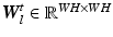 [14]
[14]
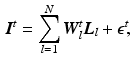
where we introduce  to account for model errors and observation noise. N is the number of layers in the image sequence. This model is justified by the log-linearity of Lambert-Beer’s law applied to X-ray attenuation. In
  , we use bilinear interpolation, but the method generalizes to other interpolation or point spread functions. Boundary treatment for image pixels moving outside of the spatial support of the layers is to take the nearest layer pixel. Alternatively, the layer support can be increased to cover all motions in the current sequence [15]. For all images and layers, the joint forward model is used

where  ,
,  , and
, and  . The system matrix
  is composed of matrices
  to transform all layers to a certain point in time.
. The transformation of a layer by its motion and subsequent interpolation is modeled in the system matrix [14](1)
to account for model errors and observation noise. N is the number of layers in the image sequence. This model is justified by the log-linearity of Lambert-Beer’s law applied to X-ray attenuation. In , we use bilinear interpolation, but the method generalizes to other interpolation or point spread functions. Boundary treatment for image pixels moving outside of the spatial support of the layers is to take the nearest layer pixel. Alternatively, the layer support can be increased to cover all motions in the current sequence [15]. For all images and layers, the joint forward model is used(2)
, , and . The system matrix is composed of matrices to transform all layers to a certain point in time.2.2 Probabilistic Approach to Layer Separation
The goal of layer separation is to find the layers  given the images
  and the motions encoded in
  . From a Bayesian point of view, the observed images
  , the noise
  , and the layers
  are random variables. Assuming conditionally independent observed images, the posterior probability of the layers given the images
  is given by
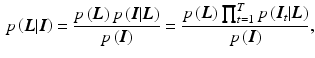
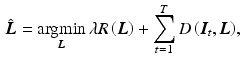
with the prior probability for the layers  and the likelihood
  for each image given the layers. Common priors in image processing are defined on local neighborhoods, such that Eq. (3) corresponds to a Markov random field. The maximum a posterior (MAP) estimate
yields the statistically optimal layers for the given model and input images. In previous work, no probabilistic motivation [3] or maximum likelihood (ML) estimation was often used [14, 17], implicitly assuming a uniform prior  .
.
given the images and the motions encoded in . From a Bayesian point of view, the observed images , the noise , and the layers are random variables. Assuming conditionally independent observed images, the posterior probability of the layers given the images is given by(3)
and the likelihood for each image given the layers. Common priors in image processing are defined on local neighborhoods, such that Eq. (3) corresponds to a Markov random field. The maximum a posterior (MAP) estimate(4)
.By applying the logarithm and negating, the probabilistic formulation can be equivalently regarded as an energy. Assuming positive values, it is possible to write prior  and likelihood
  as
as  and
and  , where
  are partition functions to normalize the probabilities. Consequently, MAP inference as in Eq. (4) turns into energy minimization
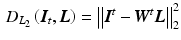
where  is the data term,
  the regularization, and
  the regularization weight. In the following sections, we concretize
  and
and  .
.
and likelihood as and , where are partition functions to normalize the probabilities. Consequently, MAP inference as in Eq. (4) turns into energy minimization(5)
is the data term, the regularization, and the regularization weight. In the following sections, we concretize and .2.3 Data Term
The data term describes how deviations from the image formation model are penalized. From a probabilistic point of view, it corresponds to an assumption on the observation noise  . The classic choice of a least-squares data term
corresponds to a Gaussian noise model, which has been used in most of the prior work [10, 14, 17] and is a fitting model for images with good photon statistics [9]. This model is easy to optimize by solving a sparse linear system of equations. Its major drawback is the sensitivity to outliers, i.e., a few erroneous measurements lead to artifacts in the estimated layers. However, outliers are very common in X-ray layer separation, for example due to errors in motion estimation, which is challenging in X-ray without knowing the layers (Sect. 2.6). Another important source of outliers is the simplified image formation model (Sect. 2.1). Many effects occurring in X-ray images are not captured by this model, e.g., foreshortening and out-of-plane motion.
. The classic choice of a least-squares data term(6)
The least absolute deviation corresponds to a Laplacian noise model
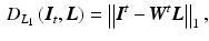
which is more robust to outliers and still a convex function. In contrast to Eq. (6), it is not smooth due to the non-differentiability at 0. Therefore, a smooth approximation to the  -norm is helpful for gradient-based optimization schemes, e.g., the Charbonnier function
 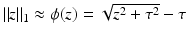 , for
, for ![$$\tau > 0$$” src=”/wp-content/uploads/2016/09/A339424_1_En_22_Chapter_IEq38.gif”></SPAN> [<CITE><A href=]() 13].
13].
(7)
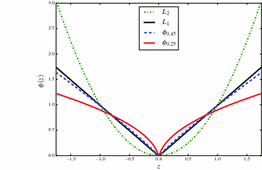
-norm is helpful for gradient-based optimization schemes, e.g., the Charbonnier function , for Fig. 1.
Behavior of different penalty functions (best viewed in color) (Color figure online).
A non-convex data term can be derived using a generalization of the Charbonnier function 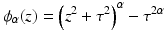 [13].
[13].  is equivalent to
  and
and  , as used in
  , is equivalent to
  . Then, the general data term is
![$$\begin{aligned} D_{\mathrm {Charb.}}\left( {\varvec{I}}_t, {\varvec{L}}\right) = \sum _{k=1}^{WH}{\phi _{\alpha }\left( \left[ {\varvec{I}}^t - {\varvec{W}}^t {\varvec{L}}\right] _k \right) }. \end{aligned}$$](/wp-content/uploads/2016/09/A339424_1_En_22_Chapter_Equ8.gif)
![$$[{\varvec{x}}]_k$$](/wp-content/uploads/2016/09/A339424_1_En_22_Chapter_IEq45.gif) extracts the k-th component of
extracts the k-th component of  . Using the generalized Charbonnier function, the value of
  can be tuned to fit the statistics of the observation noise.
  is only required for numerical reasons and set to 0.01. The penalty functions are visualized in Fig. 1. It is evident that
  and
and  are convex penalties, and that large deviations are penalized less by
  with smaller values of
  .
.
[13]. is equivalent to and , as used in , is equivalent to . Then, the general data term is(8)
extracts the k-th component of . Using the generalized Charbonnier function, the value of can be tuned to fit the statistics of the observation noise. is only required for numerical reasons and set to 0.01. The penalty functions are visualized in Fig. 1. It is evident that and are convex penalties, and that large deviations are penalized less by with smaller values of .2.4 Regularization Term
Common priors in image processing favor smoothness of the images. The most basic prior is based on Tikhonov regularization and penalizes high gradients
where  is a matrix computing the spatial derivatives for each layer. As image gradients in natural images are heavy-tailed, Eq. (9) leads to oversmoothed images. For layer separation, the
  regularization term is particularly counterproductive. Assume a certain gradient at an image location has to be represented somehow by the layers. The
  -norm gives the lowest penalty if all layers contribute equally to the image gradient. However, this corresponds to a separation into two equal layers.
(9)
is a matrix computing the spatial derivatives for each layer. As image gradients in natural images are heavy-tailed, Eq. (9) leads to oversmoothed images. For layer separation, the regularization term is particularly counterproductive. Assume a certain gradient at an image location has to be represented somehow by the layers. The -norm gives the lowest penalty if all layers contribute equally to the image gradient. However, this corresponds to a separation into two equal layers.Related posts:
 Stable Overlapping Replicator Dynamics for Multimodal Brain Subnetwork Identification
 PET Reconstruction with Sparse Image Representation and Anatomical Priors
Stay updated, free articles. Join our Telegram channel

Full access? Get Clinical Tree


