Fig. 1.
Mass spectra acquired with ∼11,000 MRP and 75 μm-width slits in front of the detectors. The analyzed cell was isotopically enriched in 13C and 15N. The ions of interest and some of the interfering isobars at m/z 13, m/z 14, m/z 26, and m/z 27 are indicated. The individual masses are not resolved in these scans, but by setting the deflection on each detector as indicated with the dashed lines, the contribution of the interfering isobars is less than 0.1% of the species of interest. Several species are too low in abundance to be visible in the mass spectra (see Table 1 for the full list of interferences at m/z 26 and 27).
Table 1
Mass Interferences
Calculated clusters | m/e (u) | Δ (mu) | Abundance | MRP |
|---|---|---|---|---|
At mass 26 | ||||
12C–14N | 26.0025 | 0.0 | 0.98538 | – |
13C–13C | 26.0062 | 3.6 | 0.00012 | 7,155 |
10B–16O | 26.0073 | 4.8 | 0.19853 | 5,443 |
1H–12C–13C | 26.0106 | 8.1 | 0.01088 | 3,208 |
1H–1H–12C–12C | 26.0151 | 12.6 | 0.97783 | 2,068 |
At mass 27 | ||||
12C–15N | 26.9996 | 0.0 | 0.00362 | – |
11B–16O | 27.0037 | 4.1 | 0.79909 | 6,567 |
13C–14N | 27.0059 | 6.3 | 0.01096 | 4,272 |
1H–12C–14N | 27.0104 | 10.8 | 0.98523 | 2,502 |
1H–13C–13C | 27.0140 | 14.4 | 0.00012 | 1,872 |
1H–1H–12C–13C | 27.0185 | 18.9 | 0.01088 | 1,429 |
1H–1H–13C–12C | 27.0185 | 18.9 | 0.01088 | 1,429 |
3.
Turn off the primary beam and move to the starting location on the target cell. Five to ten micrometers leeway should be allowed for stage drift and misalignment of the CCD and SIMS imaging.
4.
Set the analysis conditions so that the primary beam cross section from pixel to pixel overlaps by at least 50%. Scan rate is set to enable multiple scans before eroding through the plasma membrane (e.g., 512 × 512 pixels, 15 × 15 μm2, 0.5–1 ms/pixels, 3–5 scans; see below for calculation of sputter depth). Collect target species (e.g., 12C1H−, 13C1H−, 14N12C− and 15N12C−) and secondary electrons.
3.6 Data Analysis
3.6.1 Determination of Analysis Depth
Determination of the sputtering depth is straightforward, involving use of established formulas and procedures. To ensure that the vast majority of secondary ions are produced by the cell membrane and few secondary ions are collected from the underlying cytoplasm, the sputtering depth should be less than the sum of the thicknesses of the membrane (7.5 nm (21)) and the metal coating (∼5 nm). If the sputtering depth exceeds the membrane thickness, it can be reduced by discarding some of the image planes. Because the sputtering depth increases with each subsequent image plane, discard the last image plane(s) to be acquired until the sputtering depth is less than approximately 5 nm.
1.
Calculate the sputtering depth. Sputtering depth (Dsp) is calculated using the sputter rate (Rsp), primary ion beam current, at the sample (FCo) in pA, raster area (Aras) in μm2, and the sputtering time (tsp) in seconds. The sputter rate determined on other biological samples, which ranges from 0.9 nm·μm2/pA·s (unpublished results) to 2.5 nm·μm2/pA·s (10) may be employed. The primary ion beam current at FCp and raster area were recorded during NanoSIMS analysis. The primary ion beam current at the sample (FCo) must be measured separately. The sputtering time (tsp) is calculated using the dwell time (tdw) for each pixel (pxl), the total pixels (pxltot) per image plane, and the total number of image planes (NP) according to Eq. 1.
(1)
For example, for a 512 by 512 pixel image consisting of four image planes that were each acquired with a dwell of 1 ms/pixel, the total sputtering time is 1048.576 s. Calculate the sputtering depth in nanometers using Eq. 2.
(2)
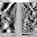
3.6.2 Determination of Lateral Spatial Resolution
Lateral resolution is also determined using standard procedures. The primary challenge is to find a sufficiently small or sharp edged feature so that its width is negligible relative to the primary beam diameter. To determine the spot size, a single scan of a standard sample is used. To determine the practical resolution, multiple scans of a cell sample can be used, but with the caveat that the features may not be sufficiently small or sharp to accurately characterize the beam diameter.
1.
Collect a secondary electron image of a standard sample (256 × 256 pixels, 5 × 5 μm2, 0.5–1 ms/pixels) or use an image that you have already collected of a cell (see above). For multi-scan images, align the NanoSIMS image planes to correct for spatial drift in the beam or the sample. The presence of image drift would compromise the lateral resolution of the resulting image. Images of high count rate species, such as 12C14N– or secondary electrons, typically provide the best alignment for cells.
2.
Calculate the effective diameter of the primary ion beam, to determine the lateral resolution of the NanoSIMS analysis. Make a line scan across a region in a secondary ion or secondary electron image where the sample composition changes abruptly. Determine the distance over which the secondary ion or electron signal intensity changes from 84% to 16% of the maximum intensity. This distance is the effective diameter of the analysis beam (7).
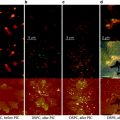
3.6.3 Creation of 15N- and 13C-Enrichment Images
To accurately visualize the distribution of 15N-sphingolipids and 13C-lipids in the plasma membrane, the secondary ion signal must be normalized to remove ion intensity variations due to concentration-independent factors that affect ion yields and sputter rates (22). These factors include changes in ionization probabilities related to sample composition—which is referred to as “matrix effects”—and sample topography (8, 23, 24). Because these concentration-independent factors influence the intensities of isotopologues, which are chemical species that differ in isotopic composition (i.e., 15N12C−, 14N13C− and 14N12C−), to relatively the same extent, expressing the lipid-specific ion counts as a ratio to the corresponding major ion accurately represents the concentration distribution of the target molecules (22). To minimize random noise in the images, the ratio images are typically “smoothed” over a 3 by 3 pixel window, which means the value at a given pixel is the average ratio of the 3 by 3 pixel region that is centered around that pixel.
1.
Align the image planes.
2.
 Introduction: Nanoimaging Techniques in Biology
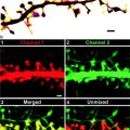 Two-Color STED Imaging of Synapses in Living Brain Slices
 Photoswitchable Fluorophores for Single-Molecule Localization Microscopy
 Functional AFM Imaging of Cellular Membranes Using Functionalized Tips
 Correlative Optical and Scanning Probe Microscopies for Mapping Interactions at Membranes
 Nanoimaging Cells Using Soft X-Ray Tomography


For each image plane, ratio the counts of each lipid-specific ion (e.g., 15N12C−or 13C1H−) detected at each pixel to the counts of the corresponding major element ion (14N12C− or 12C1H−) detected at the same pixel.
Related posts:
Introduction: Nanoimaging Techniques in Biology
Two-Color STED Imaging of Synapses in Living Brain Slices
Photoswitchable Fluorophores for Single-Molecule Localization Microscopy
Functional AFM Imaging of Cellular Membranes Using Functionalized Tips
Correlative Optical and Scanning Probe Microscopies for Mapping Interactions at Membranes
Nanoimaging Cells Using Soft X-Ray Tomography
Stay updated, free articles. Join our Telegram channel
Full access? Get Clinical Tree
