Segmentation and Discrimination of Connected Joint Bones from CT by Multi-atlas Registration

for all bone structures, while being able to accurately discriminate between neighbouring bone structures.

1 Introduction

Segmenting bone structures is of particular importance for orthopaedic surgical planning as well as implant selection and can aid in the diagnosis of pathologies such as osteoporosis, whereby the bone quality is examined, or osteoarthritis which requires an evaluation of the cartilage degradation.

Various bone segmentation methods have already been proposed with applications to segmenting the hip [1, 2], as well as the vertebrae [3, 4]. Segmenting joint bones, however, can become particularly difficult due to the thin cortex at certain regions which is exacerbated by osteoporosis. Moreover, the close proximity of the bone boundaries at the joints make it difficult to discriminate between adjacent bone structures. This in turn is aggravated by the presence of osteoarthritis, which reduces the cartilage and makes it difficult to determine where the bone ends and where the next begins. It therefore becomes necessary to include some form of a priori information into the bone segmentation method.

Statistical models have recently become popular in medical image segmentation and have already been applied to the segmentation of the proximal femur [5], the pelvic bone [6] and individual vertebrae [7]. These methods, however, often do not in a straightforward manner guarantee the separation of neighbouring bones. Moreover, the segmentation using statistical models is constrained to the main variations of the dataset used for training the model, thus not allowing the accurate segmentation of irregular pathological bones or outliers.

There has already been much research into segmenting brain structures in the field of neuroimaging where the connected brain tissue structures have to be identified and labelled to relate structural changes to neurological disorders. This is commonly done by the deformable registration of an atlas which is particularly suited to segmenting connected tissue structures as is the case with brain regions. Initially, a single-atlas registration was proposed and was later improved by the registration of multiple atlases [8], which can subsequently be merged through various combination strategies [9]. This was shown to result in segmentation accuracies exceeding all others and has rapidly become the standard in brain image segmentation.

Thus, in this work we apply the multi-atlas registration approach to the segmentation of connected joint bone structures and evaluate this technique for its ability to not only segment bone structures but also its ability to separate the connected bones. The method is evaluated for the hip whereby the proximal femur and hemipelvis are segmented and identified as well as the lumbar spine where the L2 and L3 vertebrae are individually labelled. The atlases are constructed by manual delineations of the bones and the segmentation method is evaluated in a leave-one-out analysis, giving the overlap measures and surface distances as the segmentation and discrimination accuracies.

2 Materials and Methods

2.1 Data

A dataset of 30 CT scans of the pelvic area was collected which consists of only female subjects with an average age of $43.9 \pm 14.8$ years and ranging between 20 and 78 years.¹ A dataset of lumbar spine CT scans was also collected which consists of 9 male and 21 female subjects with a mean age of $57.6 \pm 9.6$ years and ranging between 12 and 71 years.² The pelvic CT scans were performed using the Siemens Sensation 64 Slice CT system (Siemens Healthcare, Erlangen, Germany) with a pixel spacing of $0.7 \times 0.7 \mathrm{mm}$ and slice spacing of $0.5 \mathrm{mm}$ and the spinal scans using the GE LightSpeed 16 CT device (GE Healthcare, Madison, WI, USA) with a pixel spacing of $0.7 \times 0.7 \mathrm{mm}$ and slice spacing of $1.5 \, \mathrm{mm}$ . All participants gave informed consent for the analysis of their hip, pelvic and vertebral imaging data.

Fig. 1

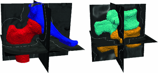
Manual segmentations of the proximal femur and hemipelvis (left) and the vertebrae (right), shown here by the surfaces extracted from the labelled tissue regions within the volumes, with the region of interest for the registration process outlined in white

For the pelvic volumes the right proximal femur was cropped below the lesser trochanter and the hemipelvis below the anterior superior iliac spine. Both the pelvic volumes and the spinal volumes were further cropped to contain only the bone structures of interest and the volumes were resampled to $1 \mathrm{mm}$ cubic voxels. In the 30 pelvic CT scans the proximal femur and hemipelvis were manually labelled as well as the L2 and L3 vertebrae in the spinal CT scans. Thus, the atlases consist of the CT volumes with associated label maps, which delineate the bone regions (Fig. 1).

2.2 Automatic Segmentation

For the automatic segmentation, the set of atlases are registered onto the target volume by means of an affine transformation followed by a multi-scale B-spline registration. For the multi-scale B-spline registration we used a control point spacing of $$32$$

and $8 \mathrm{mm}$ consecutively whereby the displacement of the control points are constrained to $$0.4$$

times the control point spacing to guarantee diffeomorphism [10]. The mutual information (MI) similarity measure was used for the registrations and a mask of the region of interest was defined by applying an appropriate threshold to the CT volume followed by a dilation to include a boundary region around the bone (Fig. 1).

The resulting transformations are applied to the corresponding label volumes using a nearest neighbour resampling, thereby propagating manual delineations from the multiple atlases to the target subject. Thus, for each of the atlases the voxels in the target volume are labelled as belonging to one of the bone structures or soft tissue.

Several common atlas combination strategies are evaluated to find one best suited for bone structures: a simple majority voting scheme, a global-weighted combination strategy, the statistical fusion method STAPLE [11] and generalized local-weighted voting. While majority voting assigns the tissue structure to each voxel based on the majority of the atlases, global weighted voting assigns a weight to each of the atlases based on the similarity between the registered atlas and the target volume. Here, the weights are determined by the mean squared error $$m$$

within the region of interest, magnified by a gain $$p$$

as $m^{p}$ .

Generalized local-weighted voting computes the weights of the atlases at each voxel separately by taking the mean squared error in a cubic neighbourhood region of diameter $$d$$

, which is again magnified by a gain $$p$$

. Since local-weighted voting can result in irregular and disconnected bone structures when incorporating a relatively small region, in a post processing step a regularization is applied to the label map. For each voxel, if a majority of neighbouring voxels is assigned to a different tissue structure, the labelling is changed to this structure. A final multi-label connected component filter is applied to fill holes in the labelled regions and remove disconnected structures, which is also applied to the segmentations from the other combination strategies, although these generally do not result in such artefacts.

2.3 Evaluation

The segmentation accuracy is evaluated by a leave-one-out method whereby for each volume the remaining 29 atlases are used for the automatic segmentation, which is then compared to the manual segmentation. The various atlas combination strategies are evaluated, as well as the use of a single-atlas where each registered atlas is considered as an individual automatic segmentation.

As a measure for the segmentation accuracy the Mean Overlap (MO) is computed:

$\begin{aligned} MO = \frac{ 2 \left| A \cap B \right| }{\left| A \right| + \left| B \right| } \end{aligned}$

(1)

where

denotes the automatic segmentation and $$B$$

the manual segmentation of the selected region. Although the Mean Overlap represents the segmentation accuracy of the individual bone structures, we are also interested in how well connected bones can be separated. Therefore, the overlap of the automatic segmentation with the manual segmentation of the neighbouring bone structure is computed as such:

$\begin{aligned} \begin{array}{lcl} FO _{femur-pelvis} &{} = &{} \left| A_{femur} \cap B_{pelvis} \right| + \left| A_{pelvis} \cap B_{femur} \right| \\ FO _{L2-L3} &{} = &{} \left| A_{L2} \cap B_{L3} \right| + \left| A_{L3} \cap B_{L2} \right| \\ \end{array} \end{aligned}$

(2)

This False Overlap (FO) measure thus evaluates how well the two bones are discriminated from each other. A value of the gain for the global weighted voting is decided upon by examining the response of these measurements to a range of values for $$p$$

. The accuracy of the local-weighted voting with respect to the MO and FO is assessed for a range of combinations of the diameter $$d$$

of the cubical neighbourhood region and the gain $$p$$

Finally, a surface mesh is extracted from the segmentations, which allows for the computation of the mean absolute Surface Distance (SD) as well as the Hausdorff distance (HD).

3 Results

For the global weighted voting a gain of $$p=-2$$

appeared to be a good compromise with respect to the MO and FO segmentation errors for the various bone structures and here this value is used for comparison with other combination strategies. In Table 1 the overlap measures and surface distances are given for all combination strategies. These results indicate that all multi-atlas strategies outperform the single-atlas segmentations method, while the generalized local-weighted voting combination strategy results in the best segmentation and discrimination for all measurements.

Table 1

The Mean Overlap (MO), False Overlap (FO, $\mathrm{mm}^3$ ), mean absolute Surface Distance (SD, mm) and Hausdorff Distances (HD, mm) for several combination strategies and the single-atlas approach