Fig. 22.1
Intima–media complex in a B-mode image of the common carotid artery (CCA). The lumen (zone Z4) is the region where the blood flows. The CCA wall is formed by the intima (zone Z1), the media (zone Z2), and the adventitia (zone Z3) regions. The interfaces between these four regions are represented by the lines LI (lumen–intima), IM (intima–media), and MA (media–adventitia)
2 Segmentation of Carotid Ultrasound Images. Brief Survey
In carotid images the challenge is to obtain accurate IMT measures. This requires the detection of both the MA and the LI boundaries. Several approaches for the segmentation of the carotid wall and IMT measurement have been published in the last two decades. A wide range of methodologies have been tested, namely, edge detection [13–19]; gray level density analysis [20]; dynamic programming [21–24]; snakes [25–36]; discrete dynamic contour and multi-scale analysis [37]; Hough transform [36, 38, 39]; template matching [40, 41]; Nakagami modeling [42]; feature extraction, fitting, and classification [43–45]; feature extraction, cubic splines, geometric contours, and dynamic programming [46, 47]; and watershed transform [48]. A fusion of different segmentation methods using an inter-greedy technique was also introduced in [49–51], but a ground truth (manual tracings) is required to estimate the errors in each iteration. A description of most of these methods can also be found in [52].
2.1 Edge Detection
In 1998, Pignoli and Longo published the first computer-assisted method for the segmentation of 2D B-mode images of the carotid [13]. This method detects the edges of the vessel structure when moving from the lumen to the far wall. The edges corresponding to the LI and MA interfaces were used to measure the IMT. In [14], Touboul et al. used a similar approach and proved that semiautomatic computer-aided segmentation reduces the intra and inter-observer variability.
An edge detection based method was used by Selzer et al. [15, 16] to make IMT measurements and to evaluate their variability over time. The operator uses the mouse to identify a few points along the LI and the MA interfaces, over the first frame of a set of successive image frames. The artery interfaces in the first frame are then detected by searching for the edges in the vicinity of the smooth curves that pass through the identified points. The same procedure is repeated for the subsequent frames, using as guides the LI and MA interfaces detected on the preceding frame. The process may require manual correction of detection errors.
Another approach based on edge detection was proposed by Liguori et al. [18], where a statistical thresholding was used to reduce the noise before computing the intensity gradient. A manual selection of the region of interest (ROI) is required.
In [17], Stein et al. used an edge detection method to prove that computer-aided IMT measurements are faster, more reproducible, and more accurate when compared to manual measurements. The ROI must contain a portion of the lumen and the corresponding intimal, medial, and adventitial layers. The operator defines the length of the ROI and manually identifies a point in the lumen region at the left limit of this ROI. The LI and MA interfaces are then detected automatically. Manual corrections are performed by editing the boundaries incorrectly detected.
One of the most accurate edge detection approaches was introduced by Faita et al. [19]. This method improves the edge detection in the presence of noise by using a first-order absolute moment edge operator (FOAM) and a pattern recognition approach. This approach also has the advantage of being real time. However, it has two important limitations. First, the difficulty in processing vessels that are curved or non-horizontal in the image axis. Second, it needs a manual selection of the ROI.
2.2 Gray Level Density Analysis
In [20], Gariepy et al. used a computerized method, based on gray level intensity and tissue recognition, to demonstrate a strong correlation between ultrasonic and histological IMT measurements and to prove that hypertension is associated with an abnormal increase of the IMT in large arteries. Patients with plaque were excluded from the study to avoid disruptions of the double line arterial pattern. The ROI was selected manually and consisted of a rectangle containing the far wall segment to analyze. The method detects the LI interface of both walls and the MA interface of the far wall. These interfaces were used to compute the average lumen diameter and the average IMT at the far wall. The computerized method was not evaluated against any manual tracings. It was used mainly to reduce the intra-observer variability.
2.3 Dynamic Programming
Gustavsson et al. [21] and Wendelhag et al. [22] proposed related dynamic programming procedures for the automatic detection of the carotid boundaries in B-mode images. Their approach linearly combines measurements of local intensity, intensity gradient, and boundary continuity into a cost function. Low values of the cost function are associated with pixels of the desired boundaries and high values are associated with other pixels. The weights of the three terms of the cost function (intensity, gradient, and continuity) were estimated in a training phase, using manual tracings as the ground truth. The procedure is completely automatic but allows the interaction of the operator in order to correct erroneous detections. To reduce the computational burden, Liang et al. [23] introduced a multi-scale version of the dynamic programming scheme proposed in [22]. The global position of the artery is computed for the coarser scale and iteratively refined down to the finer scale. The main disadvantages of these methods are the need for a training phase and the fact that the systems may need to be retrained when the scanner or its settings are changed.
More recently, a different approach based on dynamic programming was introduced in [24]. The instantaneous coefficient of variation (ICOV) was used to improve the edge detection in ultrasound images, where the noise has a multiplicative nature. The ICOV-based edge detection, the intensity gradient, robust statistics, and the a priori knowledge about the spatial distribution of the artery boundaries are used to compute fuzzy score maps for the LI and MA interfaces. These score maps are then passed to a dynamic programming procedure that computes the contour with the largest accumulated score, for each interface. The method is able to detect the LI and the MA interfaces at near and far walls, for both healthy and atherosclerotic arteries, with a wide range of plaque types and sizes. But results are significantly better for the far wall, where the automatic detection shows an accuracy similar to manual detections. The main disadvantages are the need for a manual selection of the ROI and for a training phase.
2.4 Snakes
Traditional snakes are often attracted by the wrong boundaries due to the influence of noise. In order to overcome this limitation and prevent the trapping of the snake in between the LI and the MA interfaces, Cheng et al. [25, 27] used a more robust formulation of the snake’s external energy. A manual initialization of the snake is required. In another study [26], the same authors showed that using the contours estimated by their snake-based method, instead of manual tracings, significantly reduces the intra-observer and inter-observer variability.
Loizou et al. [28–30] showed that results obtained with snake-based methods can be improved if the snake is preceded by intensity normalization and despeckling of the image. The intensity normalization consists in setting the intensity median of the lumen region to a value between 0 and 5 and the intensity median of the adventitia layer to a value between 180 and 190. The best despeckling method found consisted in iterating five times a linear scaling filter, based on statistics taken from 7 × 7 pixel windows. Both the intensity normalization and the snake initialization require user interaction. The authors presented a large statistical validation of their results against manual tracings.
Delsanto et al. [32, 34] proposed a completely user-independent scheme that combines local statistics and a snake. Local statistics were used, first, to locate the carotid artery lumen, followed by a snake-based detection of the LI and MA interfaces. It was assumed that pixels associated with neighborhoods with low intensity mean and standard deviation usually belong to the lumen. So, the lumen was located by clustering the image into two classes, by separating the pixels with those two properties from all the remaining pixels. The threshold for the mean and the one for the standard deviation were both determined empirically, using a bidimensional histogram representing the intensity standard deviation as a function of the intensity mean, computed over 10 × 10 pixel windows. Once the lumen region is located, the adventitia layers are estimated by searching below the lumen, along each image column, for the intensity peak above a given threshold. The contour that links these intensity maxima in the longitudinal direction is used to initialize the snake that refines the estimate of the MA interface. A similar procedure is followed in the detection of the LI interface, but using the largest intensity peaks between the lumen and the MA interface to initialize the snake. The method was validated against manual tracings, showing good results. However, there are several parameters that were chosen empirically, the computational burden is too high for real-time applications and the noise caused wrong detections in 10% of the cases. An improvement of this method was proposed by the same authors in [31, 33], where the near wall and diseased vessel were also processed. Three clusters were considered: (i) lumen; (ii) intima and media layers; (iii) adventitia layer. The clustering was implemented using a fuzzy K-means classifier. The boundary between class (i) and class (ii) was taken as the initial guess for the LI interface while the boundary between class (ii) and class (iii) was the initial guess for the MA interface. These boundaries were used to initialize snakes that refined the estimates of the LI and MA interfaces. The chapter reports an improvement of the IMT measurement error, as well as robustness in segmenting plaques, although with worse results for echolucent ones. The method failed in 8% of the images due to low signal-to-noise ratio or to failure of the ROI selection. A more recent version of the same approach [35] was tested on a set of 200 images acquired with three different ultrasound scanners. It was demonstrated that the segmentation performance did not depend on the scanner used. An improvement of the IMT measurement error was reported, when compared to the initial version of the method.
2.5 Discrete Dynamic Contour and Multi-scale
In [37], Gutierrez et al. used a discrete dynamic contour in a multi-scale scheme to automatically detect the carotid boundaries in B-mode images. The contour evolution was implemented as a function of a linear combination of three weighted forces: (1) an internal force, proportional to the curvature of the contour; (2) an external force, equal to the local magnitude of the intensity gradient; (3) and a damping force, proportional to the velocity of each vertex of the contour. The results showed a low accuracy in the IMT measurements.
2.6 Hough Transform
Golemati et al. [38, 39] proposed a scheme based on the Hough transform. The LI and MA boundaries are assumed to be straight horizontal lines in longitudinal sections and circular lines in transversal sections. The method is completely automatic, it is real time and both longitudinal and transversal sections of the carotid artery can be segmented. However, the need for straight horizontal or circular LI and MA interfaces is a serious limitation, since the appearance of these boundaries is often irregular. Another disadvantage is the large number of parameters that are set empirically. A normalization of the ultrasound images is required in order to minimize the variability introduced by different operators, scanners, and gain settings. More recently, the same authors [36] introduced a snake-based refinement of the carotid boundaries in transversal sections, where the snakes are initialized by the circles computed by the Hough transform approach. The results were validated using receiver operating characteristics (ROC) analysis measures between automatic contours and manual tracings.
2.7 Template Matching
Rossi et al. [40, 41] introduced an interesting parametric template matching approach for the automatic lumen detection in longitudinal sections of the CCA. The LI and MA interfaces are not computed because the method was conceived to estimate only the location of the lumen. But this technique may be useful as a first step for complete automation of the LI and MA detection, since it avoids the need for a manual location of the lumen. To decrease the computational load, the image columns are decimated. The proposed template matching scheme is based on a priori knowledge of the expected diameter range and of the typical intensity pattern of the arterial wall–lumen complex. Spatial and temporal clustering is performed over a sequence of frames in order to reject incorrect estimates. The method is real time but a training phase is required. The performance of the method is generally high but it may fall significantly when the jugular vein is present or when the signal-to-noise ratio in the lumen region is low. The algorithm was validated by comparing the lumen center positions estimated automatically with the ones traced by an operator, taken as the reference positions. The automatic recognition was considered correct if it did not deviate more than 2 mm from the reference position.
2.8 Nakagami Modeling
Destrempes et al. [42] used a segmentation scheme based on stochastic optimization that assumes the Nakagami model for the intensity distributions in a small ROI containing the CCA wall. The lumen and the adventitia were associated with the distributions with the lower and the higher means, respectively. The intima–media complex was considered the mixture. Although a good performance was reported, this approach may be of little use for images containing pathological structures, like plaque, where the assumptions about the statistical distributions of the wall layers may not be valid. For example, in the presence of a calcified plaque, the adventitia layer may not be the one with the highest mean. Another disadvantage is the need for manual initialization.
2.9 Feature Extraction, Fitting, and Classification
An integrated approach, consisting of feature extraction, fitting, and classification, was proposed by Molinari et al. [43, 44]. The authors divided the technique into two main steps: (1) the automatic location of the CCA; (2) the detection of the LI and MA interfaces of the far wall. The first step begins with the location of the seed points, defined as the local intensity maxima above a given threshold, in each image column. Line segments are fitted to these seed points. Close and aligned segments are fused while the other segments are eliminated, producing an estimate of the location of the adventitia layer. In the second step, a fuzzy K-means classifier is applied to the intensity profile of each image column, in order to assign the pixels to the lumen, to the intima–media structure, or to the adventitia layer. The boundaries that separate these three clusters were taken as the estimates of the LI and the MA interfaces. There is also a preprocessing block that uses a low pass filter to reduce speckle. A large validation against manual tracings showed a very accurate detection of the MA interface but a poor detection of the LI interface. Another disadvantage is the need for a training phase in the first step.
More recently, the same authors [45] introduced an improved version of this approach, where the detection of the LI and MA interfaces, in the second step of the method, is based on the FOAM edge operator previously used by Faita et al. [19]. This approach was validated against manual tracings on a database of 300 carotid images from two different institutions, producing very accurate detections for both LI and MA interfaces of the far wall. The authors reported an average computation time of 2.3 s per image and a failure rate of 4%.
2.10 Watershed Transform
In [48], Molinari et al. adopted an approach similar to the one used in [43, 44], but using an algorithm based on watershed transform in the CCA location step. After erosion with a 12 pixel disk-shaped structuring element, the image was reconstructed against the original one. A black and white image was computed through thresholding and the white areas were used to perform marker-based watershed segmentation. The CCA location was then selected as the segmented image region with the greater value of an ad hoc score function. The CCA region includes the lumen and the walls of the artery, but the lumen is much darker and larger than the walls. When present, the jugular vein has similar properties, but appears above the CCA. Therefore, the score function was made proportional to the percentage of dark pixels in the region and inversely proportional to the average region intensity and the average region height. The method was tested against manual tracings. The failure rate reported for this method (9.5%) was only slightly lower than the one reported for the approach presented in [43, 44]. The evaluation in a database of 165 images showed some improvement of the accuracy when compared to the one reported in [43, 44], but a lower accuracy compared to the one found in [45]. The average segmentation time per image was equal to 18 s.
2.11 Limitations of the Current Solutions
The methods described above present several important limitations. Semiautomatic approaches [13–22, 24–30, 37, 42] are not suited for the treatment of large databases and the results are affected by the user interaction. Several automatic methods are computationally heavy [31–35, 43, 44, 48], making them unattractive for clinical practice. Some studies [13–16, 20, 21, 25, 27, 37] do not consider the segmentation of plaques. Few studies [18, 24, 31, 33, 46, 47] measure the IMT at the near wall.
There are already a few commercial systems available for the IMT measurement, namely, Vivid 7, created by General Electrics (http://www.vivid7ultrasound.com); SonoCalc IMT, commercialized by SonoSite (http://www.sonosite.com); and M’Ath from Intelligence in Medical Technologies (http://www.iimt.fr). These systems compute a set of IMT measurements, like the mean and maximum, over the specified section. But they also have some limitations. For instance, they all require user interaction. Vivid 7 and Sono-Calc require the manual selection of a rectangular ROI containing the section of the artery wall where the IMT is to be measured. M’Ath requires the user to draw a longitudinal line inside the lumen in order to locate the lumen and to define the section of the wall to be segmented. They only work properly if the boundaries to detect are well visible in the specified section of the wall. Also, at least in the case of M’Ath, this section cannot include plaque.
3 Cubic Splines and Dynamic Programming for Carotid Image Segmentation
The proposed method for the segmentation of the NW and FW intima–media regions of the CCA in B-mode ultrasound images begins with an edge detection step. The final edge map is made by the edges that are compatible with the carotid wall boundaries to be detected. The MA interface is detected by a RANSAC search for the best fit of a cubic spline to edges having features compatible with the MA boundary. Several discriminating features of the MA interface are used to reduce the attraction of the automatic contour by other edges. A smooth estimate of the LI interface is obtained using dynamic programming, smooth intensity thresholding surfaces, and geometric snakes.
3.1 Edge Estimation
The edge estimation consists in the determination of an edge map representing the set of the pixels whose properties (e.g., the gradient orientation) are compatible with the carotid wall boundaries to be detected. These edges are estimated in four steps: edge detection (Sect. 3.1.1); estimation of the dominant gradient direction at edges (Sect. 3.1.2); determination of the final edge map (Sect. 3.1.3); and determination of the valley edge map (Sect. 3.1.4).
3.1.1 Edge Detection
In [46, 47], a new smoothing filter was proposed for the edge detection in B-mode images. This filter smoothes out the noise while producing well-localized edges and preserving important weak boundaries. It takes advantage of the instantaneous coefficient of variation (ICOV) edge detector [53, 54], which is well adapted to US images. The ICOV value at pixel (x,y) is computed by (22.1), using the intensities of the pixels in its 8-neighborhood.
(22.1)
In (22.1), I(x,y) represents the image intensity at (x,y), ∇I(x,y) is the intensity gradient at (x,y), and  is the norm of a vector (u,v). As explained in [53], the ICOV is an edge detector for speckled images that combines a normalized gradient magnitude operator and a normalized Laplacian. At edge pixels, the Laplacian term becomes zero, the gradient term becomes dominant, and
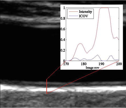
  . This normalization of the gradient magnitude allows the ICOV to detect edges both in bright regions and in dark regions, in images with multiplicative noise. As shown in Fig. 22.2, the ICOV produces local maxima at the points associated with edge pixels, where the intensity changes more rapidly.
is the norm of a vector (u,v). As explained in [53], the ICOV is an edge detector for speckled images that combines a normalized gradient magnitude operator and a normalized Laplacian. At edge pixels, the Laplacian term becomes zero, the gradient term becomes dominant, and . This normalization of the gradient magnitude allows the ICOV to detect edges both in bright regions and in dark regions, in images with multiplicative noise. As shown in Fig. 22.2, the ICOV produces local maxima at the points associated with edge pixels, where the intensity changes more rapidly.Fig. 22.2
Intensity and corresponding ICOV profiles along the line segment represented as a red line over a B-mode image
As in [55], robust statistics is used to decide where diffusion should take place and where it should be inhibited. The diffusion coefficient at pixel (x,y) and time t is a Tukey’s function [56], given by
![$$ c(x,y;t)=\left\{ {\begin{array}{*{20}{l}} {\frac{1}{2}{{{\left[ {1-{{{\left( {\frac{{\mathrm{ICOV}(x,y;t)}}{{{\sigma_s}(t)}}} \right)}}^2}} \right]}}^2}} \hfill & {,\quad \mathrm{ICOV}<{\sigma_s}} \hfill \\ 0 \hfill & {,\quad \mathrm{ICOV}\geq {\sigma_s}} \hfill \\ \end{array}} \right. $$](/wp-content/uploads/2016/08/A271459_1_En_22_Chapter_Equ00222.gif)
where  and σ e is the image edge scale [55], computed as
where MAD represents the median absolute deviation,  is the median of r over the image domain, Ω, and C = 1.4826 is a constant.
(22.2)
and σ e is the image edge scale [55], computed as(22.3)
is the median of r over the image domain, Ω, and C = 1.4826 is a constant.The proposed filter has the advantage of preserving some important anatomical boundaries even when they have a low ICOV. It is based on concepts from the total variation theory [57, 58] and embeds the curvature information, as described by
where c(x,y;t) is the Tukey’s function given by (22.2), ∇I is the intensity gradient, I 0 is the initial image, at time t = 0, ∂Ω is the image boundary, and  is the outward normal at the image boundary. κ(x,y) is the mean curvature, updated at each time step, given by
(22.4)
is the outward normal at the image boundary. κ(x,y) is the mean curvature, updated at each time step, given by(22.5)
With this filter, the diffusion is inhibited both where the ICOV is high and where the curvature is small. This way, since the LI and MA boundaries usually have low curvature, they can be preserved even when they have a low ICOV. The noise is strongly smoothed out because it usually has high curvature and low ICOV. Figure 22.3 shows the improvement introduced by this new filter when compared with a related filter previously proposed in [55]. Figure 22.3cc shows the erosion of weak edges produced by the filter proposed in [55]. Figure 22.3ee shows that the new filter is better at preserving the carotid wall boundaries.
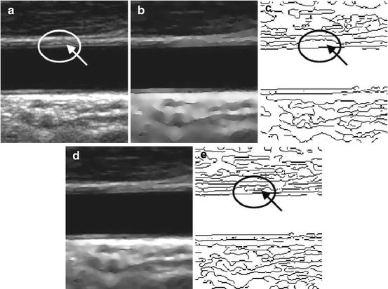
Fig. 22.3
Edge maps produced by nonlinear filtering: (a) a longitudinal section of a CCA and weak valley edges pointed out by an arrow; (b) smoothed image obtained with the filter proposed in [55]; (c) edge map of image (b) showing erosion of weak valley edges; (d) smoothed image obtained with the filter proposed in [46, 47]; (e) edge map of image (d) showing a better preservation of weak valley edges
The edge map is computed from the smoothed version of the image produced by the new filter, using the ICOV as a measure of the edge strength, non-maxima suppression, and hysteresis [59]. The lower threshold for the hysteresis was set to T 1 = σ e and the higher threshold was set to T 2 = 0.4T 1. Morphological thinning [60] is applied to the edge map to make sure the edges are one pixel thick.
3.1.2 Dominant Gradient Direction
In [46, 47], the gradient orientation errors were reduced by using the local dominant gradient direction, computed as follows. Let  be the intensity gradient at pixel (x,y), in iteration n, and
  the gradient at the kth pixel in the 8-neighborhood of (x,y), in iteration n − 1. Then
  is computed as the average of
  , for k = 1, 2,…, 9, considering only the neighbors whose gradient makes an angle less than 45° with the gradient at the central pixel, to avoid the interference of close contours with very different orientations.
be the intensity gradient at pixel (x,y), in iteration n, and the gradient at the kth pixel in the 8-neighborhood of (x,y), in iteration n − 1. Then is computed as the average of , for k = 1, 2,…, 9, considering only the neighbors whose gradient makes an angle less than 45° with the gradient at the central pixel, to avoid the interference of close contours with very different orientations.The stopping criterion of this iterative procedure was based on the stability of the gradient orientation. Let α be the angle change in the gradient orientation between consecutive iterations, at each edge pixel. Outliers can be defined as the edge pixels whose value of α does not stabilize. The threshold,  , above which no inliers of α are expected can be estimated as
  [56], where
  is a statistically robust estimate of the threshold at which the outliers start to appear [55]. Therefore, iterations stop when
  , setting ε = 0.1° in order to insure a good stability to all inliers.
, above which no inliers of α are expected can be estimated as [56], where is a statistically robust estimate of the threshold at which the outliers start to appear [55]. Therefore, iterations stop when , setting ε = 0.1° in order to insure a good stability to all inliers.3.1.3 Final Edge Map
The final edge map is determined by selecting only the edges that are compatible with the carotid wall boundaries to be detected, using criteria based on their gradient orientation, their distance to the lumen axis, and their signed distance to the lumen boundary (SDL) value. The elimination of incompatible edges reduces the computational cost and the chances of the automatic contour being attracted to other edges.
Since the gradient is expected to point outward at the carotid wall boundaries, edges with gradients pointing to the interior of the artery should be removed. If γ(x,y) is the angle, at (x,y), between the intensity gradient and the gradient of the distance map to the estimated medial axis, all edge pixels for which γ(x,y) < γ max are removed from the edge map, where γ max is the threshold above which the probability of finding an edge of the carotid MA interface is virtually zero.
All edges in the ROI whose distance to the lumen axis is larger than a certain threshold, d max, or such that SDLmin < SDL < SDLmax are also removed from the edge map.
3.1.4 Valley Edge Map
The MA interface is often associated with a valley-shaped intensity profile (Fig. 22.4), called “double line” pattern [10].
Fig. 22.4
Typical intensity profile of a valley edge, where I is the intensity, e is the location of the edge, d e is the distance from the edge in the direction of its intensity gradient, ∇I(e), a is the location of the lower peak, b is the location of the higher peak, and L is the maximum distance of search
As explained in [46, 47], the valley edge map is a subset of the final edge map described in Sect. 3.1.3. The determination of the valley edge map begins with a search, up to a certain distance, L, for the first local intensity maximum (Fig. 22.4) in both directions along the line defined by each edge point, e, and the corresponding intensity gradient, ∇I(e). The intensity profile of a valley edge has two intensity peaks, at locations a and b, one of these being usually lower. Only profiles with a strong lower peak should be classified as valley edges. Using hysteresis, as in Sect. 3.1.1, and representing the amplitude of the lower peak by A, the high threshold can be set to T A = CMAD(A) + med(A) and the low threshold to 0.4T A . However, experimentation showed that valley edge detection is better if an edge pixel is classified as a valley edge when A > 0.4T A .
3.2 Estimation of the Media–Adventitia Interface Using RANSAC
The method proposed in [46, 47] for the segmentation of the MA boundary is based on a RANSAC search for the best fit of a cubic spline [61] model according to a specified cost function. The RANSAC algorithm allows for the estimation of the model parameters from a dataset containing a large number of outliers. It works by repeatedly extracting a random sample, with the minimum number of data points required to determine the model parameters. The consensus of the model is then evaluated for the rest of the population and the model with the best consensus is selected. The process is terminated when there is a high confidence in having drawn at least one good sample.
The cubic spline [61] model was chosen for the MA boundary because it gives smooth curves, it is relatively easy to implement, it offers a stable behavior, and the results showed that it is able to adequately follow the MA interface in longitudinal sections. A dedicated gain function was conceived to evaluate the spline consensus.
3.2.1 Sample Generation and the Adventitia Model
In longitudinal sections of the CCA, samples of the MA edges must have different abscissas. Therefore, a set of n different abscissas is randomly drawn and used to determine n vertical lines above and below the lumen axis, separately. Good abscissas are those for which the corresponding vertical line contains a good point, that is, an edge point of the MA boundary.
To detect the NW MA, a cubic spline is built from each sample of n edge points with different abscissas, above the lumen axis. Since there are usually several edge points for each abscissa, the algorithm evaluates all the splines fitted to the samples of n edge points for each sample of n abscissas. The best spline, according to a predefined criterion, is then selected. A similar procedure is used for the detection of the FW MA interface. Setting n = 5 gives some flexibility to the spline without compromising its robustness to noise.
3.2.2 Model Consensus
The consensus of the fitted spline is measured by a gain function integrating the response to several discriminating features of the carotid boundaries.
Related posts:
 Relationship Between Plaque Echogenicity and Atherosclerosis Biomarkers
 Quantitative Magnetic Resonance Analysis in the Assessment of Cardiac Diseases
 Quantitative Computed Tomography Analysis in the Assessment of Coronary Artery Disease
 Visualization of Atherosclerotic Coronary Plaque by Using Optical Coherence Tomography
 Hypothesis Validation of Far Wall Brightness in Carotid Artery Ultrasound for Feature-Based IMT Measurement Using a Combination of Level Set Segmentation and Registration
 Carotid Plaque Stress Analysis: Issues on Patient-Specific Modeling
Stay updated, free articles. Join our Telegram channel

Full access? Get Clinical Tree


