Segmentation of the Spinal Cord Using Continuous Max Flow with Cross-sectional Similarity Prior and Tubularity Features

denote the intensity non uniformity corrected image [8] with intensities in the normalized intensity space $\mathcal {I}=[0,1]$ , where $x=(x_{1},x_{2},x_{3})^{\mathsf {T}}\in \Omega$ are the coordinates in the continuous image domain $\Omega \subset \mathbb {R}^{3}.$ Throughout the whole section, we furthermore assume that the tubular structure of interest is roughly oriented parallel to the $x_{3}$ axis. Figuring out the orientation should be straightforward for most clinical applications, as the subject’s orientation with respect to the image can be determined from the image’s meta data for most clinical imaging modalities.

Original max-flow formulation. A general formulation for the continuous max-flow problem with spatial flow

, source flow $p_{s}(x)$ , sink flow $p_{t}(x)$ , and corresponding flow capacities

$C_{s}(x)$ , $C_{t}(x)$ is stated by Yuan et al. [6] as

$\begin{aligned} \max _{p_{s},p_{t},p}\int \limits _{\Omega }p_{s}{\mathrm{{d}}}{x}, \end{aligned}$

(1)

subject to the flow capacity constraints

$\begin{aligned} p_{s}(x)\le C_{s}(x),\quad p_{t}(x)\le C_{t}(x),\quad \left\| p(x)\right\| \le C(x) \end{aligned}$

(2)

and the flow conservation constraint

$\begin{aligned} {{\mathrm{div}}}\, p(x)-p_{s}(x)+p_{t}(x)=0. \end{aligned}$

(3)

2.1 Cross-Sectional Similarity Prior

Following our goal to impose a cross-sectional similarity prior on the segmentation, we split the spatial flow

into an in-slice component $q:\Omega \rightarrow \mathbb {R}^{2}$ and a through-slice component $r:\Omega \rightarrow \mathbb {R}$ with respect to slices that lie perpendicular to the $x_{3}$ axis (see Fig. 1a). The resulting continuous max-flow problem can then be written as follows:

$\begin{aligned} \max _{p_{s},p_{t},q,r}\int \limits _{\Omega }p_{s}{{\mathrm{{d}}}}{x}, \end{aligned}$

(4)

subject to the new flow capacity constraints

$\begin{aligned} p_{s}(x)\le C_{s}(x),\quad p_{t}(x)\le C_{t}(x),\quad \left\| q(x)\right\| \le \alpha (x),\quad |r(x)|\le \beta (x) \end{aligned}$

(5)

and the new flow conservation constraint

$\begin{aligned} {{\mathrm{{{\mathrm{div}}}_{{12}}}}}q(x)+r^{\prime }(x)-p_{s}(x)+p_{t}(x)=0, \end{aligned}$

(6)

where ${{\mathrm{{{\mathrm{div}}}_{{12}}}}}q$ denotes the divergence of

perpendicular to the $x_{3}$ axis and $r^{\prime }$ denotes the derivative of

along the $x_{3}$ axis.

Fig. 1

Method overview. a Proposed flow configuration: the spatial flow is split into an in-slice component $$q$$

, perpendicular to the axis along which the tubular structure is oriented, and a through-slice component $$r$$

, parallel to the axis. b Sample sagittal slice of one of the images used for evaluation. c Segmentation result. d Surface reconstruction with cutting planes for volume measurement

The flow formulation now possesses the desired property of having the spatial flow capacity

of [6] represented by two separate terms, namely the in-slice flow capacity $\alpha (x)$ and the through-slice flow capacity $\beta (x)$ . The latter capacity, $\beta (x)$ , represents the cross-sectional similarity prior that allows for precise control over the through-slice flow behavior: For example, we may choose an edge-based cost function for $\alpha (x)$ that drives the segmentation towards edges in

, while setting $\beta (x)=\beta _{0}$ to enforce constant similarity throughout all slices. Or we may calculate $\beta (x)=\beta (x_{3})$ as a slice wise cost-function that, for each slice, adjusts the similarity prior to the in-slice noise level (reinforcing the similarity prior if the noise level is high and relaxing it if the noise level is low). Other combinations are possible, of course: note that both $\alpha$ and $\beta$ may be formulated pointwise.

Dual formulation. Introducing the Lagrange multiplier

and following the steps in [6], the max-flow problem can be reformulated as the equivalent primal-dual model

$\begin{aligned} \max _{p_{s},p_{t},q,r}\min _{u}\int \limits _{\Omega }p_{s}{\mathrm{{d}}}{x}+\int \limits _{\Omega }u\cdot ({{\mathrm{{{\mathrm{div}}}_{{12}}}}}q+r^{\prime }-p_{s}+p_{t}){\mathrm{{d}}}{x} \end{aligned}$

(7)

subject to the capacity constraints (5). The equivalent dual model representing a relaxed min-cut problem then becomes

$\begin{aligned} \min _{u\in [0,1]}E(u)\mathbin {:=}\int \limits _{\Omega }\left\{ (1-u)C_{s}+uC_{t}+\alpha |{{\mathrm{\nabla _{{12}}}}}u|+\beta |u^{\prime }|\right\} {\mathrm{{d}}}{x}. \end{aligned}$

(8)

Here, ${{\mathrm{\nabla _{{12}}}}}u$ denotes the in-slice gradient and $u^{\prime }$ denotes the through-slice derivative of

with respect to the $x_{3}$ axis, similar to the definitions of ${{\mathrm{{{\mathrm{div}}}_{{12}}}}}q$ and $r^{\prime }$ above. It can be shown that each level set function $u^{\ell }(x),\,\ell \in (0,1]$ given by

$$$\begin{aligned} u^{\ell }(x)\mathbin {:=}{\left\{ \begin{array}{ll} 1, &{} u^{*}(x)>\ell \\ 0, &{} u^{*}(x)\le \ell \end{array}\right. }\quad {\text {with}}\quad u^{*}\mathbin {:=}\mathop {\mathrm{{argmin}}}\limits _{u}E(u) \end{aligned}$$” src=”/wp-content/uploads/2016/10/A331518_1_En_10_Chapter_Equ9.gif”></DIV></DIV><br /> <DIV class=EquationNumber>(9)</DIV></DIV>is a global binary solution of the adapted problem stated in Eq. (<SPAN class=InternalRef><A href=$ 4).

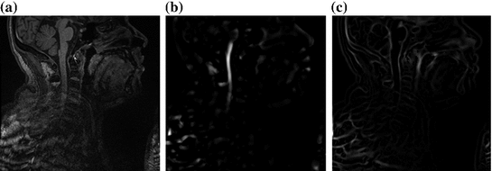
Fig. 2

Features used in segmentation. a Image intensities. b Vesselness response. c Csfness response

2.2 Tubularity Features

As our goal is to segment tubular structures in the image, it appears natural to include tubularity features in the flow capacity calculations. A well-known tubularity feature is Frangi’s measure of vesselness [9] (see Fig. 2b), $v^{*}(x)=\max _{\xi \in S_{v}}v(x;\xi )$ , where, for each scale $\xi$ in the predefined set of scales $S_{v}$ , the vesselness $v(x;\xi )$ of bright tubular structures on dark background is

$\begin{aligned} v(x;\xi )={\left\{ \begin{array}{ll} 0,\qquad \lambda _{2}\ge 0\vee \lambda _{3}\ge 0\\ \left( 1-\exp (-2\frac{\lambda _{2}^{2}}{\lambda _{3}^{2}})\right) \exp (-2\frac{\lambda _{1}^{2}}{\lambda _{2}\lambda _{3}})\left( 1-\exp (-\frac{\sum _{i=1}^{3}\lambda _{i}^{2}}{2h^{2}})\right) \quad {\text {else}}, \end{array}\right. } \end{aligned}$

(10)

with $\lambda _{i}=\lambda _{i}(x)$ denoting the ordered eigenvalues ( $\left| \lambda _{1}\right| \le \left| \lambda _{2}\right| \le \left| \lambda _{3}\right|$ ) of the pointwise Hessian matrices that result from convolving the input image $$I$$

with Gaussian derivatives of standard deviation $\xi$ . We define $$h$$

as half of the maximum Hessian norm at the current scale as suggested by Frangi [9].

In our experiments on segmenting the spinal cord, we decided to include another feature that specifically describes the background that immediately surrounds the target structure. The spinal cord is embedded in cerebrospinal fluid (CSF), which appears dark in the used MR sequences. As the CSF also appears largely elongated, but exhibits both tube-like and plate-like properties, we adapt Frangi’s vesselness feature to a csfness feature $w^{*}(x)$ (see Fig. 2c) that discriminates between blob-like structures and non-blobs. We do so by replacing the eigenvalue ratio terms of $v^{*}$ with an equivalent term composed of $\lambda _{1}$ and $\lambda _{3}$ , as it is the latter ratio that discriminates both vessels and plates from blobs in Hessian eigenvalue analysis [9]. Consequently, we define $w^{*}(x)=\max _{\xi \in S_{w}}w(x;\xi )$ for dark non-blobs on bright background in the scales $S_{w}$ with

$\begin{aligned} w(x;\xi )={\left\{ \begin{array}{ll} 0, &{} \lambda _{3}\le 0\\ \exp (-2\frac{\lambda _{1}^{2}}{\lambda _{3}^{2}})\left( 1-\exp (-\frac{\sum _{i=1}^{3}\lambda _{i}^{2}}{2h^{2}})\right) &{} {\text {else}}. \end{array}\right. } \end{aligned}$

(11)

Combining the features. Let $\mathcal {V}=[0,1]\ni v^{*}$ , $\mathcal {W}=[0,1]\ni w^{*}$ be the vesselness and csfness feature spaces, let $\mathcal {Y}=\mathcal {I}\times \mathcal {V\subset \mathbb {R}}^{2}$ and $\mathcal {Z}=\mathcal {I}\times \mathcal {V}\times \mathcal {W}\subset \mathbb {R}^{3}$ be two combined feature spaces, let $I_{2}:\Omega \rightarrow \mathcal {Y}$ , $I_{3}:\Omega \rightarrow \mathcal {Z}$ be two new image functions that map to the combined feature spaces, and let $y\in \mathcal {Y}$ , $z\in \mathcal {Z}$ be the coordinates in the combined feature spaces.