Fig. 1.
Multi-scale CNN architecture used in our experiments. One stack of three pairs of convolution (Conv) and max-pooling layers (MP) uses input image patches of size  . The second stack comprises two pairs of convolution and max-pooling layers and uses input image patches of size
  (centered at the same position). The resulting outputs
  of the k pairs of convolution
  and max-pooling
  layers are the inputs for the succeeding layers, with corresponding convolution filter sizes
  and sizes of the pooling regions
  . Our CNN also comprises two fully connected layers (FC) and a terminal classification layer (CL). The outputs of both stacks are connected densely with all neurons of the first fully-connected layer. The location parameters are fed jointly with the activations of the second fully-connected layer into the classification layer.
. The second stack comprises two pairs of convolution and max-pooling layers and uses input image patches of size (centered at the same position). The resulting outputs of the k pairs of convolution and max-pooling layers are the inputs for the succeeding layers, with corresponding convolution filter sizes and sizes of the pooling regions . Our CNN also comprises two fully connected layers (FC) and a terminal classification layer (CL). The outputs of both stacks are connected densely with all neurons of the first fully-connected layer. The location parameters are fed jointly with the activations of the second fully-connected layer into the classification layer.2.1 Representing Inputs and Targets
The overall data comprises M tuples of medical imaging data, corresponding clinical reports and voxel-wise ground-truth class labels  , with
  , where
  is an intensity image (e.g., a slice of an SD-OCT volume scan of the retina) of size
  ,
,  is an array of the same size containing the corresponding ground-truth class labels and
  is the corresponding textual report. During training we are only given
  and train a classifier to predict
  from
from  on new testing data. In this paper we propose a weakly supervised learning approach using semantic descriptions, where the voxel-level ground-truth class labels
  are not used for training but only for evaluation of the voxel-wise prediction accuracy.
, with , where is an intensity image (e.g., a slice of an SD-OCT volume scan of the retina) of size , is an array of the same size containing the corresponding ground-truth class labels and is the corresponding textual report. During training we are only given and train a classifier to predict from on new testing data. In this paper we propose a weakly supervised learning approach using semantic descriptions, where the voxel-level ground-truth class labels are not used for training but only for evaluation of the voxel-wise prediction accuracy.Visual and Coordinate Input Information. To capture visual information at different levels of detail we extract small square-shaped image patches  of size
  and larger square-shaped image patches
  of size
  with
with  centered at the same spatial position
  in volume
  , where i is the index of the centroid of the image patch. For each image patch, we provide two additional quantitative location parameters to the network: (i) the 3D spatial coordinates
  of the centroid i of the image patches and (ii) the Euclidean distance
  of the patch center i to a given reference structure (in our case: fovea) within the volume. We do not need to integrate these location parameters in the deep feature representation computation but inject them below the classification layer by concatenating the location parameters and activations of the fully-connected layer representing visual information (see Fig. 1). The same input information is provided for all experiments.
of size and larger square-shaped image patches of size with centered at the same spatial position in volume , where i is the index of the centroid of the image patch. For each image patch, we provide two additional quantitative location parameters to the network: (i) the 3D spatial coordinates of the centroid i of the image patches and (ii) the Euclidean distance of the patch center i to a given reference structure (in our case: fovea) within the volume. We do not need to integrate these location parameters in the deep feature representation computation but inject them below the classification layer by concatenating the location parameters and activations of the fully-connected layer representing visual information (see Fig. 1). The same input information is provided for all experiments.Semantic Target Labels. We assume that objects (e.g. pathology) are reported together with a textual description of their approximate spatial location. Thus a report  consists of K pairs of text snippets
  , with
  , where
  describes the occurrence of a specific object class term and
  represents the semantic description of its spatial locations. These spatial locations can be both abstract subregions (e.g., centrally located) of the volume or concrete anatomical structures. Note that
  does not contain quantitative values, and we do not know the link between these descriptions and image coordinate information. This semantic information can come in
  orthogonal semantic groups (e.g., in (1) the lowest layer and (2) close to the fovea). That is, different groups represent different location concepts found in clinical reports. The extraction of these pairs from the textual document is based on semantic parsing [15] and is not subject of this paper. We decompose the textual report
  into the corresponding semantic target label
  , with
 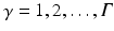 , where K is the number of different object classes which should be classified (e.g. cyst), and
  is the number of nominal region classes in one semantic group
  of descriptions (e.g.,
  for upper vs. central vs. lower layer,
  for close vs. far from reference structure). I.e., lets assume we have two groups, then
  is a K-fold concatenation of pairs of a binary layer group
  with
with  bits representing different layer classes and a binary reference location group
  with
with  bits representing relative locations to a reference structure. For all object classes, all bits of the layer group, and all bits of the reference location group are set to 1, if they are mentioned mutually with the respective object class in the textual report. All bits of the corresponding layer group and all bits of the corresponding reference location group are set to 0, where the respective object class is not mentioned in the report. The vector
  of semantic target labels is assigned to all input tuples
  extracted from the corresponding volume
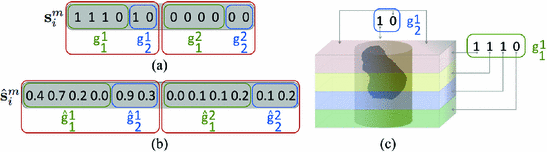
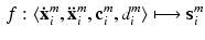
  . Figure 2a shows an example of a semantic target label representation comprising two object classes. According to this binary representation the first object is mentioned mutually with layer classes 1, 2 and 3 and with reference location class 1 in the textual report. Figure 2c shows the corresponding volume information.
consists of K pairs of text snippets , with , where describes the occurrence of a specific object class term and represents the semantic description of its spatial locations. These spatial locations can be both abstract subregions (e.g., centrally located) of the volume or concrete anatomical structures. Note that does not contain quantitative values, and we do not know the link between these descriptions and image coordinate information. This semantic information can come in orthogonal semantic groups (e.g., in (1) the lowest layer and (2) close to the fovea). That is, different groups represent different location concepts found in clinical reports. The extraction of these pairs from the textual document is based on semantic parsing [15] and is not subject of this paper. We decompose the textual report into the corresponding semantic target label , with , where K is the number of different object classes which should be classified (e.g. cyst), and is the number of nominal region classes in one semantic group of descriptions (e.g., for upper vs. central vs. lower layer, for close vs. far from reference structure). I.e., lets assume we have two groups, then is a K-fold concatenation of pairs of a binary layer group with bits representing different layer classes and a binary reference location group with bits representing relative locations to a reference structure. For all object classes, all bits of the layer group, and all bits of the reference location group are set to 1, if they are mentioned mutually with the respective object class in the textual report. All bits of the corresponding layer group and all bits of the corresponding reference location group are set to 0, where the respective object class is not mentioned in the report. The vector of semantic target labels is assigned to all input tuples extracted from the corresponding volume . Figure 2a shows an example of a semantic target label representation comprising two object classes. According to this binary representation the first object is mentioned mutually with layer classes 1, 2 and 3 and with reference location class 1 in the textual report. Figure 2c shows the corresponding volume information.Fig. 2.
(a) Example of a semantic target label comprising two object classes (K = 2). Each of which comprises a layer group  with 4 bits (layer 1,2,3, or 4) and a reference location group
  with 2 bits (close or distant). (b) Prediction of a semantic description
  that would lead to a corresponding object class label prediction
  . (c) Visualization of the volume information which could lead to the given semantic target label shown in (a). (Best viewed in color) (Colour figure online)
with 4 bits (layer 1,2,3, or 4) and a reference location group with 2 bits (close or distant). (b) Prediction of a semantic description that would lead to a corresponding object class label prediction . (c) Visualization of the volume information which could lead to the given semantic target label shown in (a). (Best viewed in color) (Colour figure online)Voxel-wise Ground Truth Labels. To evaluate the algorithm, we use the ground-truth class label  from
from  at the center position
  of the patches for every multi-scale image patch pair
  . Labels include the reported observations
  and a healthy background label.
  is assigned to the whole multi-scale image patch pair
  centered at voxel position i.
from at the center position of the patches for every multi-scale image patch pair . Labels include the reported observations and a healthy background label. is assigned to the whole multi-scale image patch pair centered at voxel position i.2.2 Training to Predict Semantic Descriptors
We train a CNN to predict the semantic description from the imaging data and the corresponding location information provided for the patch center voxels. We use tuples 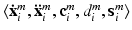 for weakly supervised training of our model. The training objective is to learn the mapping
 Stable Overlapping Replicator Dynamics for Multimodal Brain Subnetwork Identification
 PET Reconstruction with Sparse Image Representation and Anatomical Priors
 Method to Discover Genetically Driven Image Biomarkers
 Segmentation and Registration Through the Duality of Congealing and Maximum Likelihood Estimate
 Tumor Growth Prediction with Multiplicative Growth and Image-Derived Motion
 Frames for Heart Fiber Reconstruction


for weakly supervised training of our model. The training objective is to learn the mappingRelated posts:
Stable Overlapping Replicator Dynamics for Multimodal Brain Subnetwork Identification
PET Reconstruction with Sparse Image Representation and Anatomical Priors
Method to Discover Genetically Driven Image Biomarkers
Stay updated, free articles. Join our Telegram channel
Full access? Get Clinical Tree
