); 192 slices in sagittal orientation were acquired with an in-slice resolution of  and a slice thickness of 1 mm. The phantom was scanned in 11 different
  -positions relative to the magnetic field center (
 to 50 mm in increments of 10 mm). The manufacturer’s three-dimensional distortion correction routine was applied to the data to see the effects of image distortions induced by gradient non-linearity [7]. Both original and corrected datasets were reconstructed.
To assess the scan–rescan reliability, 12 healthy volunteers (3 female, 9 male, mean age 32.4 y, range 26–44 y) were scanned on a 3T whole-body MR scanner (Verio, Siemens Medical, Germany) with a T1-weighted MPRAGE sequence (TR/TI/TE/ ); 192 slices in sagittal orientation parallel to the interhemispheric fissure were acquired with an isotropic resolution of
  . Both original and distortion-corrected datasets were reconstructed.
); 192 slices in sagittal orientation parallel to the interhemispheric fissure were acquired with an isotropic resolution of . Both original and distortion-corrected datasets were reconstructed.To show the applicability to clinical data, 12 relapsing-remitting MS patients (8 female, 4 male, mean age 32.2 y, range 21–46 y; mean disease duration 8.2 y, range 1–17 y, median EDSS 3.0, range 1–4) and 12 age-matched controls (6 female, 6 male, mean age 31.6 y, range 22–48 y) were scanned on a 3T whole-body MR scanner (Verio, Siemens Medical, Germany) with a T1-weighted MPRAGE sequence (TR/TI/TE/ ); 192 slices in sagittal orientation parallel to the interhemispheric fissure were acquired with an isotropic resolution of
  . Distortion-corrected datasets were reconstructed.
); 192 slices in sagittal orientation parallel to the interhemispheric fissure were acquired with an isotropic resolution of . Distortion-corrected datasets were reconstructed.3 Method
The proposed method can be broken down into four distinct steps, which we refer to as presegmentation, segmentation refinement, surface reconstruction, and reformatting. Of these steps, only presegmentation and reformatting need manual intervention while the others run in a completely automated manner. In this way, the user interaction time lies in the order of two to five minutes per scan.
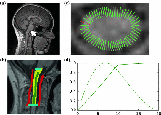
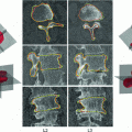
Fig. 1
a Location of the cisterna pontis. b Presegmentation (blue region of interest, red background seeds, green cord seeds, yellow result). c  d Refinement: c intensity profile locations, d single intensity profile (solid) with smooth derivative estimate (dashed), both normalized for display
d Refinement: c intensity profile locations, d single intensity profile (solid) with smooth derivative estimate (dashed), both normalized for display 3.1 Presegmentation
The aim of the presegmentation step (see Fig. 1b) is to gain a binary voxel mask that roughly separates the SC section of interest from the background; that is, from the surrounding cerebrospinal fluid (CSF) and all non-cord tissue. While in principle any kind of thresholding technique could be applied, we use graph cuts [3] because of their flexibility and speed. To compensate for intensity differences caused by field inhomogeneities, we apply a bias field correction [11] to the image volumes beforehand. Furthermore, we normalize the image intensities to the ![$$[0,1]$$](/wp-content/uploads/2016/03/A323246_1_En_13_Chapter_IEq10.gif) interval. We then build a six-connected graph from the voxels around the region of interest (which the user may sketch in transverse, sagittal, and coronal projections of the image volume).
interval. We then build a six-connected graph from the voxels around the region of interest (which the user may sketch in transverse, sagittal, and coronal projections of the image volume).
interval. We then build a six-connected graph from the voxels around the region of interest (which the user may sketch in transverse, sagittal, and coronal projections of the image volume).The t-link weights are calculated based on a naive Bayes classifier via the intensity distributions of a set of foreground and background seed points; that is, a selection of voxels labeled by the user as definitely belonging either to the SC or its surroundings. We model the foreground as a univariate normal distribution and the background as a mixture of four Gaussians. More specifically, we calculate the weights  and
and  for the t-links that connect voxel
  to the foreground and background terminal, respectively, as
 where
where  and
and  are the sets of foreground and background seed points,
  is the intensity of voxel
  , and
, and  and
and  are the probability density functions that we estimated from the foreground and background seed point intensities.
and for the t-links that connect voxel to the foreground and background terminal, respectively, as and are the sets of foreground and background seed points, is the intensity of voxel , and and are the probability density functions that we estimated from the foreground and background seed point intensities.The n-link weights  between neighboring voxels
  and
and  are calculated as
  , where
  and
and  are the respective voxel intensities,
  is a weighting factor, and
  determines the spread of the Gaussian-shaped function (with smaller values for
  leading to a faster decrease of
  for increasing differences
  ). The presegmentation is concluded by connected-component labeling, assuring that only the region that includes foreground seeds is retained.
between neighboring voxels and are calculated as , where and are the respective voxel intensities, is a weighting factor, and determines the spread of the Gaussian-shaped function (with smaller values for leading to a faster decrease of for increasing differences ). The presegmentation is concluded by connected-component labeling, assuring that only the region that includes foreground seeds is retained.3.2 Segmentation Refinement
Let  denote the preprocessed (i.e., bias field corrected) image, and let
  denote the voxel indices in the image domain
  . Furthermore, let
  denote the set of foreground mask voxel indices from the presegmentation step. To reduce noise in
  , we apply the GradientAnisotropicDiffusionImageFilter of ITK1 with the conductance parameter fixed to
  , the time step fixed to
  , and the number of iterations fixed to
  and
and  for the image used in the first and second pass, respectively. In this way, we yield the denoised images
  and
and  .
.
denote the preprocessed (i.e., bias field corrected) image, and let denote the voxel indices in the image domain . Furthermore, let denote the set of foreground mask voxel indices from the presegmentation step. To reduce noise in , we apply the GradientAnisotropicDiffusionImageFilter of ITK1 with the conductance parameter fixed to , the time step fixed to , and the number of iterations fixed to and for the image used in the first and second pass, respectively. In this way, we yield the denoised images and .In the first pass, for each transversal slice, we determine the mask boundary voxel indices  as
as
where  denotes the morphological erosion operator,
  is the two-dimensional structuring element representing four-connectivity, and
  is the subset of mask voxels for the
  -th transversal slice.
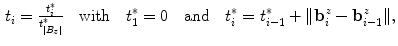
as(1)
denotes the morphological erosion operator, is the two-dimensional structuring element representing four-connectivity, and is the subset of mask voxels for the -th transversal slice.We then fit a periodic smoothing B-spline [5]  of degree three through the ordered voxel indices
  . We distribute the spline’s knots
 ![$$t_{i}\in [0,1]$$](/wp-content/uploads/2016/03/A323246_1_En_13_Chapter_IEq49.gif) (
( ) according to
and constrain the spline smoothness by a smoothing parameter  via
via
The order of the boundary voxels  is determined by calculating an estimate of their centroid as
 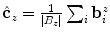 and then sorting them according to the angles formed by the
  -axis and the vectors
  . Once we have
  , we divide it into
  sections of equal arc length, yielding
  new vertices
  (
( ) at the section endpoints. For each
  , we then extract a one-dimensional intensity profile (see Fig. 1c+d)
  with
with ![$$x\in [0\ldots k_{1}-1]$$](/wp-content/uploads/2016/03/A323246_1_En_13_Chapter_IEq63.gif) as
as

where  denotes the unit normal vector pointing inside the spline curve at
  , the resampling distance is given via
  , the number of profile samples via
  , and
, and  is an offset to control the profile centering with respect to
  , yielding offset-corrected vertices
  . As our approach to calculate
  systematically underestimates the mask boundary by half a voxel, we set
  . To get the intensity values at the resampling positions
  , we use bilinear interpolation in the
  th transversal slice of
  .
.
of degree three through the ordered voxel indices . We distribute the spline’s knots () according to(2)
via(3)
is determined by calculating an estimate of their centroid as and then sorting them according to the angles formed by the -axis and the vectors . Once we have , we divide it into sections of equal arc length, yielding new vertices () at the section endpoints. For each , we then extract a one-dimensional intensity profile (see Fig. 1c+d) with as(4)
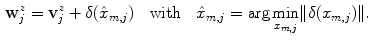
denotes the unit normal vector pointing inside the spline curve at , the resampling distance is given via , the number of profile samples via , and is an offset to control the profile centering with respect to , yielding offset-corrected vertices . As our approach to calculate systematically underestimates the mask boundary by half a voxel, we set . To get the intensity values at the resampling positions , we use bilinear interpolation in the th transversal slice of .Given that the extracted profiles point to the inside of the spline curve and knowing that in T1-weighted images the inside (i.e., the SC tissue) typically appears brighter than its immediate surroundings (i.e., the CSF), we try to refine the  by means of edge detection in the profiles
  . We thus calculate their derivatives as
 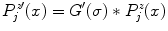 , where
  is the spatial derivative of a Gaussian kernel with standard deviation
  and zero mean. We then search for all local maxima
  in
in  and calculate the new boundary estimate
  as
as
To be less susceptible to noise, we dismiss all  with
with 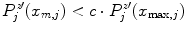 beforehand, where
 ![$$c\in [0,1]$$](/wp-content/uploads/2016/03/A323246_1_En_13_Chapter_IEq86.gif) serves as a threshold and
serves as a threshold and  is the global maximum position of
  . If no valid maxima are retained, which may be the case if the global maximum value is negative, we set
  .
.
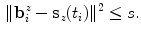
by means of edge detection in the profiles . We thus calculate their derivatives as , where is the spatial derivative of a Gaussian kernel with standard deviation and zero mean. We then search for all local maxima in and calculate the new boundary estimate as(5)
with beforehand, where serves as a threshold and is the global maximum position of . If no valid maxima are retained, which may be the case if the global maximum value is negative, we set .A second pass of boundary estimation follows, similar to the first pass, starting with the  as initial estimate. The only differences are the following: first, to ensure a homogeneous distribution of the boundary estimates, particularly with regard to the surface reconstruction step (Sect. 3.3), the fitted spline is now resampled
  times at equal angular distances, using the spline center as point of reference, yielding redistributed estimates
 Monitoring of Syndesmophyte Growth in Ankylosing Spondylitis Using Computed Tomography
 Robust Segmentation Framework for Spine Trauma Diagnosis
 Detection and Labelling in Lumbar MR Images
 of Spinal Deformities Using a Parametric Torsion Estimator
 Based Tensor Level Set Framework for Vertebral Body Segmentation
 Segmentation and Discrimination of Connected Joint Bones from CT by Multi-atlas Registration


as initial estimate. The only differences are the following: first, to ensure a homogeneous distribution of the boundary estimates, particularly with regard to the surface reconstruction step (Sect. 3.3), the fitted spline is now resampled times at equal angular distances, using the spline center as point of reference, yielding redistributed estimates
Related posts:
Robust Segmentation Framework for Spine Trauma Diagnosis
Based Tensor Level Set Framework for Vertebral Body Segmentation
Stay updated, free articles. Join our Telegram channel
Full access? Get Clinical Tree
