Fig. 1.
Top-left : Original image. Top-right : Image affected by CTF with no envelope decay. Bottom-left : Image affected by CTF with envelope decay (the decay acts as a lowpass filter). Bottom-right : Image affected by CTF with envelope decay and noise.
In this chapter, we introduce the standard image processing workflow needed to produce a volume from a collection of micrographs. The workflow is presented with the use of Xmipp 3.0 software. Note that other software packages may define different workflows, but in any case, the final structure of a complex must be obtained through a user-defined sequence of the standard steps introduced in this chapter.
In short, the standard image processing workflow starts by screening the micrographs to check that they are not astigmatic or drifted and realize the maximum frequency available. Then particles are selected from the micrographs either manually or semiautomatically. Particles are extracted from the micrographs into a gallery and they are again screened to find possible wrongly picked particles. The set of selected particles is aligned and classified attempting to identify possible 2D inhomogeneities. Possible contaminants or alternative structures are removed from the dataset. Next, an initial model is constructed either from the particles themselves or from a priori knowledge about the particle being reconstructed. Finally, the initial model is further refined using the projection images and its resolution estimated. At this level of model refinement it is still possible to have a mixture of different structural populations, and there are methods to sort them into different homogeneous classes.
2 Materials
1.
Software. SPA image processing is normally performed via software packages like Spider (4), Eman (5), Imagic (6), or Xmipp (7) among others. These software suites allow image processing starting from the raw micrographs and ending at the final reconstructed three-dimensional (3D) structure (see Note 1).
2.
Hardware. The whole process is rather demanding of computational resources and it is normally performed in computer clusters or supercomputers (cloud computing is an obvious choice for the future but at present it is not in place). The operating system of this kind of computers is always Unix-like, and therefore, Unix is the natural environment for these software packages. An average configuration of Xmipp uses a cluster with 8–16 Gb of RAM memory per node, 8–32 cores per node, and several nodes. Most Xmipp programs scale well up to 128 processors. Beyond this point, inter-process communications and disk access may become a bottleneck, although the optimal performance is rather system dependent and has to be tested on each cluster configuration.
3 Methods
In the following, we describe the mainstream protocols needed to perform a 3D reconstruction starting from the electron micrographs.
3.1 Micrograph Screening
The first step is to check the quality of the collected micrographs. Only high-quality micrographs should progress to further analysis in a high-resolution analysis. For medium-low resolution analysis, one might include not so good micrographs depending on the resolution loss that one is willing to tolerate. The Xmipp protocols produce a number of criteria that may help to screen good from bad micrographs.
3.1.1 Identifying Astigmatic and Drifted Micrographs
Good micrographs have a homogeneous background level (without any smooth gradient along the micrograph), are not astigmatic, have no drift, and have high-resolution structural information (visible Thon rings in high frequencies) (see Fig. 2). Astigmatic micrographs could, in principle, be processed. However, in practice they are avoided since most programs cannot track correctly the astigmatism angle through all the sequence of iterative alignments.
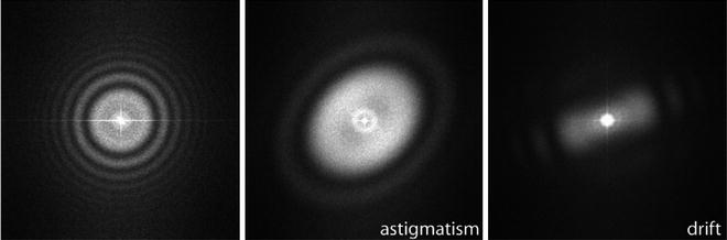
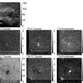
Fig. 2.
Left : Example of a good micrograph, the PSD has circularly symmetric Thon rings. The presence of many Thon rings is normally associated to the preservation of structural information in high frequency. Middle : Example of astigmatic micrograph, Thon rings are elliptical. Right: Example of drifted micrograph, Thon rings appear incomplete.
Micrographs can be semi-automatically screened by estimating their Power Spectrum Density (PSD) and their Contrast Transfer Function (CTF) (8). The PSD is an estimate of the energy distribution of the micrograph over frequency. Astigmatic micrographs have elliptical rings, while non-astigmatic micrographs have circular rings. Drifted micrographs have masked Thon rings (they do not appear to be complete). The CTF is normally described by a number of parameters, among which the most important are the microscope operating voltage and the defocus (9). However, Xmipp provides a full 2D characterization of the CTF, as well as, the background noise (8), which also plays a role in the accurate determination of the defoci and cannot simply be “filtered out.”
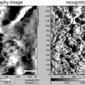
In order to correctly estimate the PSD it is important that the digital micrograph does not have empty borders or labels as in Fig. 3.
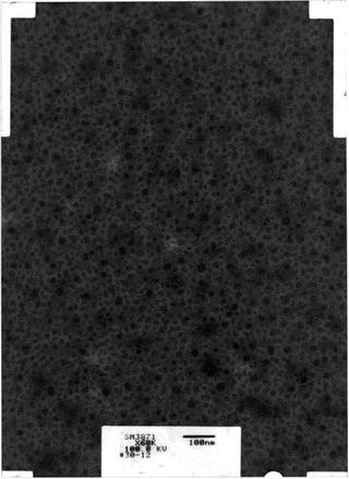
Fig. 3.
Example of digitized micrograph with blank areas in the corners and a label for identification. The PSD may not be correctly estimated if these elements are present in the digital micrograph.
3.1.2 Determining the Maximum Resolution of the Micrographs
The information content of the micrograph is an important issue to consider. We need to estimate at which resolution the information content of the micrograph fades into the noise (let us call  to this frequency). This frequency is characterized by a strong decay of the envelope of the CTF (Xmipp reports the frequency at which the CTF envelope drops below 1% of its maximum value). 3D Reconstruction algorithms may recover a few Angstroms more of resolution beyond this frequency, but not many, and the final volume resolution is strongly determined by the maximum resolution visible in the micrographs.
to this frequency). This frequency is characterized by a strong decay of the envelope of the CTF (Xmipp reports the frequency at which the CTF envelope drops below 1% of its maximum value). 3D Reconstruction algorithms may recover a few Angstroms more of resolution beyond this frequency, but not many, and the final volume resolution is strongly determined by the maximum resolution visible in the micrographs.Related to the maximum attainable resolution are the sampling rate and the downsampling factor. The sampling rate relates spatial frequencies measured in 1/Angstroms with digital frequencies measured in cycles/sample (the maximum digital frequency is 0.5 cycles/sample (10)). The relationship is w = f T, where wis the digital frequency, fis the spatial frequency in 1/Angstroms, and Tis the sampling rate in Angstroms/pixel. When we downsample the images, we increase the pixel size. Downsampling brings in two important benefits: first, images are obviously smaller with the subsequent gain in disk space and computing time; second, downsampling reduces the noise in the images by cutting out in Fourier space a region where no signal is present.
In principle, we can increase the pixel size by a factor Kas long as  (downsampling by a factor larger than this introduces an effect called aliasing in which high-frequency components may be strongly degraded). In practice, it is normally preferred to have a safety region such that
  (this is so to avoid the aliasing of the signal with the noise). For instance, if
  , and
, and  , then we can downsample by a factor
  . Note that the downsampling factor may not be an integer number. In the Xmipp protocols, downsampling is performed in Fourier space (and that is why it can accept non-integer factors). Downsampling in Fourier space provides the best accuracy even for integer downsampling factors since the micrograph PSD is multiplied by a rectangular window (11). On the other side, downsampling by simply averaging neighboring pixels (an operation often called binning) introduces strong distortions in the high-frequency components (11).
(downsampling by a factor larger than this introduces an effect called aliasing in which high-frequency components may be strongly degraded). In practice, it is normally preferred to have a safety region such that (this is so to avoid the aliasing of the signal with the noise). For instance, if , and , then we can downsample by a factor . Note that the downsampling factor may not be an integer number. In the Xmipp protocols, downsampling is performed in Fourier space (and that is why it can accept non-integer factors). Downsampling in Fourier space provides the best accuracy even for integer downsampling factors since the micrograph PSD is multiplied by a rectangular window (11). On the other side, downsampling by simply averaging neighboring pixels (an operation often called binning) introduces strong distortions in the high-frequency components (11).Considering  (
( being the effective sampling rate after downsampling), ideal micrographs have
  . Micrographs with
  (also called oversampled) can be safely downsampled since no special gain in resolution will be obtained by so finely sampled images and the noise present may hinder the quality of the final reconstruction. Micrographs with
  may suffer from aliasing resulting in reconstruction artifacts (they are said to be undersampled).
(being the effective sampling rate after downsampling), ideal micrographs have . Micrographs with (also called oversampled) can be safely downsampled since no special gain in resolution will be obtained by so finely sampled images and the noise present may hinder the quality of the final reconstruction. Micrographs with may suffer from aliasing resulting in reconstruction artifacts (they are said to be undersampled).3.1.3 Criteria to Identify Bad Micrographs Based Only on the Micrograph PSD
1.
PSD correlation at 90°. The PSD of non-astigmatic micrographs correlates well with itself after rotating the micrograph 90°. This is so because non-astigmatic PSDs are circularly symmetrical, while astigmatic micrographs are elliptically symmetrical. High correlation when rotating 90° is an indicator of non-astigmatism. In Xmipp, this criterion is computed on the enhanced PSD (12).
2.
PSD radial integral. This criterion reports the integral of the radially symmetrized PSD. This criterion can highlight differences among the background noises of micrographs. This criterion is computed on the enhanced PSD.
3.
PSD variance. The PSD is actually estimated by averaging different PSD local estimates in small regions of the micrograph. This criterion measures the variance of the different PSD local estimates. Untilted micrographs have equal defoci all over the micrograph, and therefore, the variance is due only to noise. However, tilted micrographs have an increased PSD variance since different regions of the micrograph have different defoci. Low variance of the PSD is indicative of non-tilted micrographs.
4.
PSD Principal Component Variance. When considering the local PSDs previously defined as vectors in a multidimensional space, we can compute the variance of their projection onto the first principal component axis. Low variance of this projection is indicative of a uniformity of local PSDs, for example, this is another measure of the presence of tilt in the micrograph.
5.
PSD PCA Runs test. When computing the projections onto the first principal component, as discussed in the previous criterion, one should expect that the sign of the projection is random for untilted micrographs. Micrographs with a marked nonrandom pattern of projections are indicative of tilted micrographs. The larger the value of this criterion, the less random the pattern is.
3.1.4 Criteria to Identify Incorrectly Fitted CTFs
1.
Fitting score. The CTF is computed by fitting a theoretical model to the experimentally observed PSD. This criterion is the fitting score. Smaller scores correspond to better fits. A complete description of Xmipp fitting score is given at Sorzano, Jonic (8).
2.
Fitting correlation between the first and third zeroes. The region between the first and third zeroes is particularly important since it is where the Thon rings are most visible. This criterion reports the correlation between the experimental and theoretical PSDs within this region. High correlations indicate good fits.
3.
First zero disagreement. If the CTF has been estimated by two different methods (normally Xmipp and Ctffind (13)), then this criterion measures the average disagreement in Angstroms between the first zero in the two estimates. Low disagreements are indicative of a correct fit.
3.1.5 Criteria to Identify Bad Micrographs Based on the Fitted CTF
1.
Damping. This is the envelope value at the border of the PSD. Micrographs with a high envelope value at border are either wrongly estimated or strongly undersampled.
2.
First zero average. This is the average in Angstroms of the first zero over all possible directions. Normally, this value should be between 4 and 10 times the effective sampling rate in Angstroms/pixel.
3.
First zero ratio. This measures the astigmatism of the CTF by computing the ratio between the largest and smallest axes of the first zero ellipse. Ratios close to 1 indicate no astigmatism.
3.2 Particle Picking
The next step is to pick particles from those micrographs passing the previous screening step. Particle picking can be performed manually or semiautomatically. Manual particle picking simply lets the user to choose those particles he is interested in from the electron micrographs. The ease of picking particles depends on the particle size, image contrast, contamination level, etc. The task can be facilitated by displaying the micrograph with a moderate zoom-out factor.
Image filters can also help to better visualize the particles of interest. In Xmipp we provide the following filters: color dithering, bandpass filter, anisotropic diffusion, mean shift, background subtraction, and contrast/brightness enhancement. Particularly useful are color dithering and bandpass filtering. Color dithering (14) is an algorithm that reduces differences between adjacent gray values. Bandpass filter (15) filters out gray-scale variations that are either too small or too large with respect to the size of the particle we are interested in.
3.2.1 Manual Particle Picking
Manual picking is sometimes criticized for biasing the dataset towards those shapes that the user better recognize or has in mind as the possible projections of her structure. In order to avoid this bias, automatic or semiautomatic particle picking algorithms are sometimes preferred as an objective way of choosing particles. At the same time, the particle picking process, which in general is a tedious and time-consuming task, is computationally assisted and accelerated. Algorithmically chosen datasets contain a nonnegligible amount of wrongly picked particles (contaminants, true particles on carbon, particle conglomerates, etc.). These datasets have to be carefully scrutinized to remove wrongly picked particles from the onset. This can be done by a manual revision of the automatic picking results, and/or by classifying in 2D the selected particles and eliminating those classes corresponding to wrongly picked particles.
3.2.2 Semiautomatic Particle Picking
Xmipp allows semiautomatic particle picking (16). The algorithm has been designed to keep a low false-positive rate (FPR), i.e., picking as few wrongly picked particles as possible. In order to keep the FPR as low as possible, the algorithm must be trained by the user in the kind of particles he is interested in. The first step of the training requires the user to manually pick about 100–200 particles. Then, the algorithm learns a set of features describing the particles being picked. In the next step, the algorithm tries to automatically select particles from a micrograph that has not been manually processed. The first attempt will pick a number of true particles, but many other true particles may be left. The user is required to pick those “unseen” particles. He is also required to correct the algorithm by removing those particles that have been wrongly picked automatically. This correction information helps the algorithm to distinguish true particles from other objects looking alike. This process of the algorithm trying to correctly pick particles and the user correcting for errors is repeated on more micrographs until the user is satisfied with the algorithm results. At each step, the algorithm learns from its errors and next time it will try to better distinguish between particles and nonparticles. No automatic particle picking algorithm is absolutely infallible. As a rule of thumb, they can be applied when the imaging conditions are not specially challenging.
3.3 Particle Extraction, Screening, and Preprocessing
The next step is to extract the particles from the micrographs and form a stack of projections of our particle. This stack of projections is further analyzed in 2D or 3D in subsequent steps. Projection screening helps to identify projections that are not typical (in the statistical sense). Nontypical particles may correspond to underrepresented projection directions or states of our particle, but also to wrongly picked particles and outliers. If an automatic particle picking algorithm has been used, nontypical particles normally correspond to wrongly picked particles, such as particles on edges. Finally, particle preprocessing helps to highlight or concentrate specific features of our dataset.
3.3.1 Particle Extraction
When extracting the particle projections, there are a number of actions we can take:
1.
Phase flipping. Use the information from the estimated CTF to compensate for phase reversals introduced by the microscope at different frequencies. This phase correction is better performed on the micrographs (not the projections), since we have enough information to perform a deconvolution.
2.
Taking logarithm. Depending on your acquisition system you may have to take the logarithm of the data in order to have a linear relationship between the gray values in the image and those in the volume.
3.
Contrast inversion. Most image processing algorithms expect to see the particle as a white object over a dark background. However, some imaging conditions produce just the opposite. At this moment, you may invert the contrast if your particles are black over a white background.
4.
Normalization. The same projection in different micrographs may have different gray values. Even within the same micrograph there might be a light gradient causing the gray values to be different. In order to eliminate a local gradient, a ramp in the gray values is fitted for each projection image and then subtracted from the image. Then, the image values are linearly transformed so that in the background there is zero mean and standard deviation equal to one. Noise statistics should be similar in all projections after this normalization step.
5.
Dust removal. Sometimes dust, hot or cold spots can be seen in a projection. These pixels are identified by noting that their gray values are normally far from the mean of the rest of the image. You should choose to fill these pixels with a random value from a Gaussian with zero-mean and unity-standard deviation.
3.3.2 Particle Screening
Automatic picking algorithms have a nonnegligible FPR (i.e., they pick locations in the micrograph that do not actually correspond to true particles). Particle screening is a successful way of identifying them.
For each image, we calculate the gray values histogram, square the gray values and compute the radial average of these squared values. The gray histogram and the radial average are stacked into a multivariate vector associated to each projection. Now, we perform a PCA analysis of the whole set of projections and project the multivariate vector onto the PCA space spanned by the first two eigenvectors. Then, we analyze the multivariate normality of these projections. The normality is measured as the Mahalanobis distance of the PCA projection to the space origin. Typical projections have a small distance, while nontypical projections have a larger distance. The dataset is sorted according to their distance (called z-score). Normally, wrongly picked particles, particles on edges, contaminants, etc., have a large distance and are sorted to the end of the list. At this point, the user may discard the particles he considers that do not correspond to the structure under study, or that for some reason do not follow the general trend.
Related posts:
 Introduction: Nanoimaging Techniques in Biology
 Two-Color STED Imaging of Synapses in Living Brain Slices
 Secondary Ion Mass Spectrometry Imaging of Biological Membranes at High Spatial Resolution
 High Data Output Method for 3-D Correlative Light-Electron Microscopy Using Ultrathin Cryosections
 Functional AFM Imaging of Cellular Membranes Using Functionalized Tips
 Single-Molecule Tracking of mRNA in Living Cells
Stay updated, free articles. Join our Telegram channel

Full access? Get Clinical Tree


