Shape Representation for Modeling, Elastic Registration and Segmentation

defines a planar smooth curve with parameter . The cartesian coordinates of the point vector can be defined by $\mathbf{C}(p) = [x(p)y(p)]^{T}$ where $0 \le p \le 1, 0 \le x, \le X$ and $0\le y, \le Y$ . This is the explicit representation of the given shape or contour $\mathbf{C}$ . Open shapes have the relation $\mathbf{C}(0) \ne \mathbf{C}(1)$ . A closed contour will always have $\mathbf{C}(0) = \mathbf{C}(1)$ . Parameterizing complicated topology shapes is a challenge which is considered a disadvantage of the explicit shape representation method. Thus, a parametrization-free representation is needed. The implicit shape representation satisfies this condition as shown.

Given a smooth curve $\mathbf{C}^\alpha$ (defined above), that represents boundaries of the shape of interest, the following implicit vector function is defined as $\Phi _{\alpha }(\mathbf X):\Omega _{\alpha }\subset R^2 \rightarrow R^2$ where

$\begin{aligned} \Phi {\alpha }\mathbf{(X)}= \mathbf{X}_{0}-\mathbf{X}= [\phi _1\phi _2]^T, \mathbf{X}\in \Omega _{\alpha }, \phi _{1} \;and\; \phi _{2}\in R, \end{aligned}$

(1)

where $\mathbf{X}_0$ is the point on $\mathbf{C}^\alpha$ with the minimum Euclidean distance to $\mathbf{X}$ where $\mathbf{X}\in \Omega _{\alpha }$ ( $\Omega _{\alpha }$ is the domain that includes the shape/contour). The surface or boundary points always satisfy the relation $||\Phi _\alpha (\mathbf{C}^\alpha )|| = 0$ . Note, that the implicit representation is dependent only on the boundary position, not on any parameterizations, and hence, it is suitable to represent a cloud of points or even scattered edge boundaries.

If a global transformation is applied to the given shape represented by the designed vector map, one can predict the map of the new shape. We define a shape $\beta$ that is obtained by applying a transformation $\mathbf{A}$ to a given shape $\alpha$ . Let us assume that the transformation has a scale matrix $\mathbf{S}$ , a rotation matrix $\mathbf{R}$ , and a translation vector $\mathbf{T}$ . The transformation can be written for any point $\mathbf{X}$ in the space as $\mathbf{A}= \mathbf{SRX} + \mathbf{T}$ .

Applying the transformation to the given points results in the pair of points $\hat{\mathbf{X}}, \hat{\mathbf{X}}_{0} \in \Omega _\beta$ (Domain of the Target Shape where $\Omega _\beta \subset R^2$ ). It is straightforward to show that:

$\begin{aligned} \Phi _\beta (\mathbf{A}) = \hat{\mathbf{X}}_{0} - \hat{\mathbf{X}} = \mathbf{SR}(\mathbf{X}_0-\mathbf{X}) \end{aligned}$

(2)

as such the following relation holds:

$\begin{aligned} \Phi _\beta (\mathbf{A}) = \mathbf{SR}\Phi _\alpha (\mathbf {X}) \end{aligned}$

(3)

Which illustrates that this representation can give a vector similarity measure that includes inhomogeneous scales and rotations. Also, it is invariant to the translation parameters, while the effect of scales and rotations can be predicted. This measure overcomes the problem of using the conventional signed distance maps that leads to the use of homogeneous scales only. Note, that the VDF components are smooth and differentiable at the boundary points.

3 Global Registration of Shapes

Finding point-wise correspondences (between the two given source and target shapes defined respectively by $\mathbf{C}^\alpha$ and $\mathbf{C}^\beta$ ) is the objective of the registration problem. An energy function is built based on the vector dissimilarity measure. The VDF shape representation changes the problem from the shape boundary domain to the higher dimensional vector representation. A transformation, $\mathbf{A}$ , that gives pixel-wise vector correspondences between the two shape representations $\Phi _\alpha$ and $\Phi _\beta$ , is required to be estimated.The problem now can be considered as a global optimization that includes all points in the image domain. Sum of squared differences will be considered with energy optimized by the gradient descent approach.

According to the properties of the implicit vector representation shown, the following dissimilarity measure is used: $\mathbf{r} = \mathbf{SR} \Phi _{\alpha } (\mathbf{X}) - \Phi _\beta (\mathbf{A})$ and the optimization energy function is formulated by the sum of squared differences as: $E(\mathbf{S, R, T})=\mathop {\smallint }\nolimits _{\Omega \alpha }\mathbf{r}^{T}\mathbf{r}d\Omega _\alpha$ . The complexity of the problem is reduced by considering only points around the zero level of the vector function and neglecting mapping of far away points. The matching space is limited to a small band around the surface that can be selected by introducing the following energy function:

$\begin{aligned} E(\mathbf{S, R, T})=\mathop {\smallint }\nolimits _{\Omega \alpha }\delta _\varepsilon (\Phi _\alpha , \Phi _\beta )\mathbf{r}^{T}{\mathbf{r}}d\Omega _\alpha . \end{aligned}$

(4)

where $\delta _\varepsilon$ is an indicator function defined in [1].

The optimization of the given criterion is handled using the gradient descent method:

$\begin{aligned} \frac{d}{dt}\vartheta = 2\mathop {\smallint }\nolimits _{\Omega \alpha }\delta _\varepsilon \mathbf{r}^T[\nabla _\vartheta (\mathbf{SR}\Phi _\alpha (\mathbf{X})) - \nabla \Phi ^T_{\beta }(\mathbf{A})\nabla _\vartheta {\mathbf{A}}] d \Omega _\alpha \end{aligned}$

(5)

where $\vartheta \in \{S_x, S_y, \theta , T_x, T_y\}$ represents the set of scale, rotation, and translation parameters respectively.

3.1 Evaluation of Global Registration

In [10] we reported results for an experiment that involved 100 registration cases, using the corpus callosum (simple shape) and the hippocampus (four separate parts). Each case considers a source and a target shape. The source is fixed and the target is generated by applying a transformation on the source. Parameters ( $S_x, S_y, \theta , T_x, T_y$ ) are created and selected randomly from the ranges [0.8, 1.2], [0.8, 1.2], [ $-60^\circ , 60^\circ$ ], [ $$-60$$

, 60] respectively. These generated patterns are kept as the ground truth for each case. The gradient descent optimization is performed to obtain a steady state estimate for each parameter associated with each registration case. The algorithm shows successful results for the one hundred cases and the energy decreases smoothly with the increase of the iteration number until perfect alignment is achieved. The measurements show that the mean errors and standard deviations (Table 1) are very appropriate and satisfactorily small. The final registration emphasizes that for each experiment, the boundaries of the source and target shapes become very close to one another. The gradient descent successfully estimates the scales, rotations, and translations with proper initialization.

Table 1

Mean error ( $\mu$ ) and its standard deviation ( $\delta$ ) for the transformation parameters of the corpus callosum (CC) and hippocampus (HC) cases $(\mu \pm \delta )$

Structure			$\theta ^\circ$
CC	$-0.005\pm 0.009$	$-0.003\pm 0.007$	$-0.002\pm 0.018$	$-0.5\pm 0.4$	$-0.3\pm 0.5$
HC	$0.009\pm 0.007$	$0.005\pm 0.004$	$0.001\pm 0.09$	$0.00\pm 0.02$	$-0.0\pm 0.02$

Parameter ranges:[ $$0.8, 1.2$$

], [

], [ $-60^{\circ }, 60^{\circ }$ ], [ $$-60, 60$$

], [

], are used

In addition, we formed three groups of different shapes (Fighter Jet, Fishes, Number Four). Each group includes 11 instances of its corresponding shape. Different global registration processes are conducted by randomly taking 11 pairs from each group. For each pair of shapes, the correlation coefficient is calculated to measure the similarity between the shape representations: $\gamma = \frac{E[(||\Phi _\alpha ||-\mu _\alpha )(||\Phi _\beta ||-\mu _\beta )]}{\sigma _\alpha \sigma _\beta }$ where $\mu ,\sigma$ stand for mean and standard deviation of the shape vector representations magnitudes respectively. The global registration process successfully increases the coefficient dramatically. Before alignment, the mean correlation coefficients and their standard deviations for the groups are ( $0.836\pm 0.047$ ), ( $0.834\pm 0.087$ ), and ( $0.754\pm 0.092$ ), respectively. After alignment, the coefficients become ( $0.969\pm 0.013$ ), ( $0.953\pm 0.03$ ), and ( $0.911\pm 0.039$ ). Note, that the last group has the largest local shape variations and hence, has the smallest average coefficient 0.911, which is small compared to other groups of coefficients.

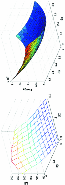
Fig. 1

Large scales registration case: the negative of mutual information is given to the left. The proposed energy is given to the right. The mutual information and the proposed energy are shown as functions of and the proposed energy are shown as functions of $$S_x$$

and

For comparison with other techniques, two synthetic shape images have been created. The second image results by stretching the first with large inhomogeneous scales ( $$S_x = 2.5, S_y = 3.3$$

). Mutual information is used to register these contours (images) according to the technique in [15]. Mutual information suffers in such a situation because the scale range will increase/decrease the energy in one direction, providing unacceptable results (minimum position does not provide the correct parameters as shown in Fig. 1 left image). The proposed approach aims to align the contours of the given images to each other to obtain a global minimum at these scales exactly as shown, which is considered to be an advantage over the mutual information.

3.2 Global Registartion for Segmentation of Lung Nodule Regions

We use the global alignment approach with the shape-based segmentation as an application. In our previous work [2], we formulated the problem as a global registration between a shape and an intensity model implicit representation. In this paper, we adopt the above alignment technique to segment lung nodule regions [16]. Nodule size is an important factor in volumetric analysis of lung nodules. It has been shown clinically that size is linked to nodule malignancy, with non-calcified nodules larger than in diameter having a higher rate of malignancy than smaller nodules. Size computation is usually performed by applying volumetric methods to a segmentation result. However, lung nodules segmentation in CT imaging is a complex and challenging process. One of the most important problems arises from possible attachments of the nodules to other anatomical objects. The lungs are a complex anatomical structure. Vessels, fissures, bronchi or pleura are structures that can be located close to lung nodules.

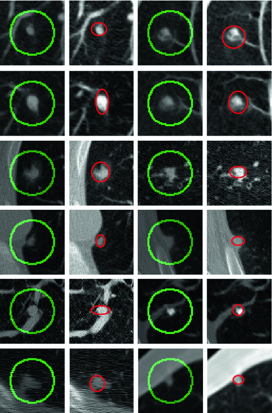
Fig. 2

Initial positions are shown in green at the first and third columns while final ellipses are demonstrated in red at the second and fourth columns

From our experience, we noticed that the main nodule regions considered for size computation are elliptic. A circle model is represented implicitly by the vector function ${{\Phi }_{\!p}}$ . A region of interest image (ROI) is taken from the whole lung CT scan to include the nodule. Intensity segmentation of the ROI is represented implicitly by the vector function $\Phi _{\!g}$ . Aligning the two models using the above approach will result in an ellipse that includes the nodule region. The model is initialized and then the alignment parameters are estimated using the gradient descent optimization. Different scales, rotation, and translation parameters are computed in each case to obtain an ellipse exactly around the nodule (see Fig. 2). The ellipse axis rotates while its size changes to include the boundaries of the nodule. A thresholding technique can be used later to remove the non-nodule parts from the elliptic areas.

4 The Elastic Registration Problem

Our objective is to find a function that gives the point correspondences between the two given domains (source and target). Let us define the 2

shape elastic registration as follows:A map $\mathbf{C}^{\hat{\alpha }}(\tau _s):[0, 1] \in R \rightarrow R^2$ defines a planar source curve with a parameter $\tau _s$ (it is the source shape $\mathbf{C}^\alpha$ after applying the global transformation estimated by the methods above). The target is defined by $\mathbf{C}^\beta (\tau _t):[0, 1] \in R \rightarrow R^2$ . Assume that $\mathbf{C}^{\hat{\alpha }}(\tau _s)$ is the corresponding point of $\mathbf{C}^\beta (\tau _t)$ (the criteria for finding the correspondences can be found in the following sections). The output will be a

function $f:R^2 \rightarrow R^2$ with $f(\mathbf{C}^{\hat{\alpha }}(\tau _s)) = \mathbf{C}^\beta (\tau _t)$ . Different interpolation functions have been proposed to handle this problem [12]. We choose the free form deformation

model, based on B-splines [13, 14], which is a powerful tool for modeling deformable objects and has been previously applied to the tracking and motion analysis problems. The basic idea is to deform the shape by manipulating a mesh of control points. The resulting deformation controls the shape of the object and produces a smooth and continuous transformation.

Consider an $M\times N$ lattice of control points $\mathbf{P} = \mathbf{P}_{m, n};m\in \{1,\ldots ,M\};n\in \{1,\ldots ,N\}$ , each point on the source shape will have the following form of deformation:

$\begin{aligned} \mathbf{L}(\tau _s) = {\sum }^3_{k=0} {\sum }^3_{l=0} B_k(u)B_l(v)\delta \mathbf{P}_{i + k, j+1} \end{aligned}$

(6)

where $\delta \mathbf{P} = \delta \mathbf{P}_{m, n}\in \{[\delta \mathbf{P}^x_{1, 1}\delta \mathbf{P}^y_{1, 1}]^T,\ldots ,[\delta \mathbf{P}^x_{M, N}\delta \mathbf{P}^y_{M, N}]^T\}$ is the control point deformation vector,

$$i=(x.(M-1)/X)+1, j = (y.(N-1)/Y)+1, u = x.M/X), v = y.N/Y - (y.N/Y)$$

, and the spline basis functions

are defined in [14]. So the cubic B-spline is used as an approximation function for our interpolation problem. Below, we propose and discuss the problem solution in implicit and explicit spaces. In [10], we devised a closed form solution of the interpolation function parameters.

4.1 A Coarse to Fine Strategy with IFFD’s

The control lattice points are required to move to correctly obtain correspondences over shape boundaries. A very small error can be achieved when using a high resolution control lattice since the number of degrees of freedom increases. However, this is not enough. Such sudden movement will result in unnecessary cross overs of the domain grid lines and the registration process will be meaningless. This will result in changing and corrupting the object topology. A better way is to move the grid step by step towards the target.

To avoid this, a coarse to fine strategy is used (equivalent to the incremental free form deformations used in [15]). We start with a resolution of $4\times 4$ and solve for the deformation. Iteratively we increase the resolution to $5\times 5, 6\times 6$ , and so on and so forth. In each step, the positions of the control points are computed and the contour moved to the new position until a satisfactory error distance is obtained. The result is smooth and the correspondence is achieved accurately. This process handles the error extremely well and provides an impressive infinitesimal energy function and smooth grid deformations simultaneously.

4.2 Solution in Vector Implicit Spaces

Following the work in [11], a local deformation vector $\mathbf{L} = \mathbf{L}(\mathbf{X}) = \mathbf{L}(\delta \mathbf{P})$ (described above) is applied to the globally transformed shape represented by $\hat{\alpha }$ . The following dissimilarity measure is considered:

$\begin{aligned} \mathbf{r}_n - \Phi _{\hat{\alpha }}(\mathbf{X}) - \Phi _\beta ({\mathbf{X+L}}) \end{aligned}$

(7)

and hence the non rigid energy function will be defined as:

$\begin{aligned} E^\Phi _n(\delta \mathbf{P}) = \mathop {\smallint }\nolimits _{\Omega _{\hat{\alpha }}}\mathbf{r}^{T}_{n}\mathbf{r}_n d\Omega _{\hat{\alpha }} \end{aligned}$

(8)

The local deformations are smoothed by adding another term that includes their derivatives as follows:

$\begin{aligned} E^\Phi _n(\delta \mathbf{P}) =&\mathop {\smallint }\nolimits _{\Omega _{\hat{\alpha }}}\mathbf{r}^T_n\mathbf{r}_n d\Omega _{\hat{\alpha }}+\lambda \mathop {\smallint }\nolimits _{\Omega _{\hat{\alpha }}}(||\mathbf{L}_x||^2+||\mathbf{L}_y||^2\nonumber \\&+||\mathbf{L}_{xx}||^2+||\mathbf{L}_{yy}||^2)d\Omega _{{\hat{\alpha }}} \end{aligned}$

(9)

As an interpretation, the energy contains a term for covering the local deformations and another for penalizing large derivatives. To make the addition homogeneous, we weight the second term by $\lambda \in R^{+}$ . Again, we take the derivative of the energy with respect to each of the unknown parameters as follows:

$\begin{aligned} \frac{\partial E^\Phi _n}{\partial \delta \mathbf{P}}&=\;-2 \mathop {\smallint }\nolimits _{\Omega _{\hat{\alpha }}}\mathbf{r}^T_n(\nabla \Phi _\beta )^T \frac{\partial \mathbf{L}}{\partial \delta \mathbf{P}}d\Omega _{{\hat{\alpha }}}+2\lambda \mathop {\smallint }\nolimits _{\Omega _{\hat{\alpha }}}((\mathbf{L}_x)^{{T} \frac{\partial \mathbf{L}_{x}}{\partial \delta \mathbf{P}}}\nonumber \\&\quad +(\mathbf{L}_{y})^{T} \frac{\partial \mathbf{L}_y}{\partial \delta \mathbf{P}} +({\mathbf{L}_{xx}})^T\frac{\partial \mathbf{L}_{xx}}{\partial \delta \mathbf{P}}+({\mathbf{L}_{yy}})^T\frac{\partial \mathbf{L}_{yy}}{\partial \delta \mathbf{P}}) d\Omega _{{\hat{\alpha }}} \end{aligned}$

(10)

We assume that the amount of pixel deformation is relatively small such that its vector representation can be approximated using Taylor series expansion as: $\Phi _{\beta }(\mathbf{X}+\mathbf{L}) \approx \Phi _{\beta }(\mathbf{X})+(\nabla \Phi _{\beta }(\mathbf{X})^{T})\mathbf{L}$ . The control points are required to move and minimize the above objective function and hence satisfy the following zero condition: $\frac{\partial E^\Phi _n}{\partial \delta \mathbf{P}} = [0\quad 0]^{T}$ . By setting $\Phi (\mathbf{{X}}) = {\Phi _{\hat{\alpha }}}(\mathbf{{X}})-\Phi _{\beta }(\mathbf{{X}})$ , the above formulation will lead to:

$\begin{aligned} \mathop {\smallint }\nolimits _{\Omega _{\hat{\alpha }}} \Phi ^{T}(\nabla \Phi _{\beta })^{T}\frac{\partial \mathbf{L}}{\partial \delta \mathbf{P}}d\Omega _{{\hat{a}}}&= \mathop {\smallint }\nolimits _{\Omega _{\hat{\alpha }}}((\nabla \Phi _{\beta })^{T}\mathbf{L})^{T}(\nabla \Phi _{\beta })^{T}\frac{\partial \mathbf{L}}{\partial \delta \mathbf{P}}d\Omega _{{\hat{a}}} \nonumber \\&\quad +\lambda \mathop {\smallint }\nolimits _{\Omega _{\hat{\alpha }}}((\mathbf{L}_{x})^{T}\frac{\partial \mathbf{L}_{x}}{\partial \delta \mathbf{P}}+(\mathbf{L }_y)^{T}\frac{\partial \mathbf{L}_{y}}{\partial \delta \mathbf{P}}+(\mathbf{L}_{xx})^{T}\frac{\partial \mathbf{L}_{xx}}{\partial \delta \mathbf{P}} \nonumber \\&\quad +\big (\mathbf{L}_{yy})^{T}\frac{\partial \mathbf{L}_{xx}}{\partial \delta \mathbf{P}}\big )d\Omega _{{\hat{a}}} \end{aligned}$