Fig. 1.
Verification for labeling of the cytoplasmic mRNA. (a) A DNA construct for the expression of the MS2-EGFP protein with an NLS. (b) DNA constructs for the expression of β-actin mRNAs with and without the MS2-bs. (c) Distribution of MS2-EGFP in a CEF expressing mRNA with an MS2-bs. An arrow and an arrowhead indicate the nucleus and the leading edge of the cell, respectively. β-actin mRNA is localized to the leading edge of the cytoplasm. (d) Distribution of MS2-EGFP in CEFs expressing mRNA without an MS2-bs. MS2-EGFP is localized to the nucleus (arrow ). The scale bars represent 10 μm (adapted from ref. 12 with the permission of Elsevier).
3.2 Quantification of the Fluorescence Intensity of each Fluorescent Spot
Cytoplasmic mRNAs will be observed as bright spots. To confirm how many mRNA molecules are present in each bright spot, it is recommended that the fluorescence intensities of individual bright spots are compared with those of single EGFP molecules.
3.2.1 Optical Setup for the Measurement of the Fluorescence Intensity
1.
For live cell imaging, use an inverted epifluorescence microscope with an incubation system, such as a stage-top incubator, to maintain the temperature of the cells at 37°C (see Note 5).
2.
Use a high magnification and high numerical aperture objective lens, such as PlanApo N TIRF (60×, NA = 1.45) oil immersion objective, to identify single spots in the cytoplasm and suitable to ensure the collection of faint fluorescence signals from single EGFP molecules.
3.
Illuminate the specimen with blue laser power of a few μW/μm2 at the sample surface. Generally, the intensity distribution of the laser beam is approximated by a Gaussian function, which will result in different efficiencies of excitation by inhomogeneous illumination. Therefore, the beam line should be expanded by a beam expander, and the intensity data should be acquired within a limited area of irradiation around the center to avoid too large a variation in the irradiation intensity (for example, within 10% variation).
4.
Place a dichroic mirror (Q505LP) and emission filter (FF01-520/35-25) combination optimal for collecting EGFP fluorescence emission in the microscope (see Note 6). An excitation filter is not required, because the introduction of an excitation filter in the laser line may cause uneven illumination owing to the interference fringe.
5.
To observe the quantized photobleaching of single EGFP molecules, acquire images at 20 frames per second, or faster, using a cooled electron-multiplying charge-coupled device (EM-CCD) camera (a cooled EM-CCD camera is best suited for quantification of the fluorescence intensity of single EGFP molecules). The electron-multiplying gain register can increase the signal more than several hundredfold before any readout noise is added, therefore keeping the noise level low. Furthermore, a cooled EM-CCD camera incorporating back illuminated type CCD chips is recommended for its high quantum efficiency (see Note 7).
3.2.2 Measurement of the Fluorescence Intensity of Single EGFP Molecules
To accurately measure the fluorescence intensity of single EGFP molecules, a purified solution of EGFP is required. The preparation method for obtaining recombinant EGFP is described elsewhere (14).
1.
Load purified EGFP at the concentration of ng/ml level in a saline solution such as PBS onto a pre-cleaned glass coverslip to be absorbed nonspecifically (see Note 8). Excess free EGFP is then washed with the saline solution prior to observation.
2.
Acquire series of images of single EGFP molecules to measure changes in fluorescent intensity before and after quantized photobleaching. We typically monitor the intensity for at least 10 s at video rate under conditions where single EGFP molecules photobleach in a few seconds on average.
3.
Measure the fluorescence intensities with select regions within the image series using image analysis software (see Note 9). The region of interest (ROI) for specifying a fluorescence molecule is made by the circle with the smallest diameter to cover the Airy disk. The ROI for calculating the background fluorescence is made by a slightly larger diameter circle. The margin between the smaller ROI and the larger ROI, which forms a concentric ring that surrounds the Airy disk, is used to calculate the background fluorescence intensity.
3.2.3 Measurement of the Fluorescence Intensity of mRNA Molecules in Living CEFs
1.
With the transfected CEFs cells on the microscope, acquire single image snapshots under the same optics and imaging conditions (optics setup, camera frame rate) as in the quantification of the intensities of single EGFP molecules (see Note 10).
2.
To analyze the fluorescence intensities of mRNA molecules in the transfected CEFs, draw ROIs the same size as those used in the quantification of the intensities of single EGFP molecules. To extract the position of bright spots in the cytoplasm of CEFs, dynamic thresholding is an effective approach and is described below.
In a previous study, we completed such an analysis from 1,354 bright spots in the cytoplasm and 352 EGFP molecules on the coverslips, and compared the distributions of fluorescence intensities using histograms (12). An average intensity of single EGFP molecules was determined from the histogram fitted with a Gaussian distribution. The histogram of intensities of bright spots was fitted with a single Gaussian distribution with the average equivalent to six molecules of EGFP (Fig. 2a), indicating that each individual spot was bound with an average of six EGFP molecules. Up to eight EGFP molecules can bind to each single β-actin-MS2-bs mRNA molecule. The determined number of EGFP molecules in the cytoplasmic spots was about the same as the expected number of GFP molecules for a single mRNA. Therefore, we conclude that the individual bright spots seen in the cytoplasm are single β-actin mRNA molecules.
Fig. 2.
Single-molecule tracking of β-actin mRNA. (a) Histogram of fluorescence intensities of single EGFP molecules (gray bars) and β-actin mRNA molecules labeled with EGFP (black bars). A solid line and a broken line indicate Gaussian distributions fitted to the data. The fluorescence intensity is normalized by the average intensity of single EGFP molecules. (b) Wide-field epifluorescence micrograph of β-actin mRNA molecules labeled with EGFP in a CEF. (c) Magnified image of the rectangular region in (b). Trajectories of 15 mRNA molecules are numbered. (d) Galleries of trajectories of mRNA molecules in the perinuclear region (No. 1–5) and at the leading edge (No. 8–15) of the cell. Nos. 6 and 7 in (c) were excluded from the analysis because they are not located in the perinuclear or leading edge regions. (e) Ensemble-averaged MSD–t plots for the perinuclear region (circles) and the leading edge (squares). Bars indicate SEM. Data were fitted with Eq. 7 (adapted from ref. 12 with the permission of Elsevier).
3.3 SMT of β-Actin mRNA Labeled with MS2-EGFP
3.3.1 Epifluorescence Microscopy for SMT
The same inverted microscope with the equipment described in Subheading 3.2.1 can be used for SMT; however, the camera setting should be reconsidered depending on the motility and spatial crowding of the target molecules. Successive images should be captured at a fast enough frequency to track each molecule of interest in the presence of high concentrations of other molecules. Otherwise the molecule of interest mixes with other molecules.
1.
Place in the laser path a field stop that corresponds to a tracking area (15 μm in diameter) at the specimen plane, so that EGFP molecules outside of the tracking area are not illuminated.
2.
Capture images of 10.6 × 10.6 μm rectangle field in the tracking area by an EM-CCD camera every 8 ms with intense laser illumination (a few μW/μm2 at the sample surface) because β-actin mRNA molecules at the leading edge of CEFs are present at a high density and they move rapidly. A large number of fluorescent spots are photobleached by the intense laser and the remaining spots decrease in density such that they can be distinguished as discrete spots. Track the remaining fluorescent spots and newly appearing fluorescent spots from outside of the illumination area.
3.3.2 Protocol of SMT
There are many software packages suitable for automated particle tracking. Some require their licenses to be purchased and some are offered by several research groups as freely downloadable files. In this article, we refer to the plug-in program for trajectory analysis running on Aquacosmos software that we have successfully used in the single mRNA molecule tracking studies. This program facilitates the definition of a target molecule position by fitting a Gaussian curve to the fluorescence intensity profile of the molecule (or calculating the centroid coordinate of the bright spot) and also searches for the nearest-positioned bright spot in the following frame as the same molecule after displacement. The plug-in program for trajectory analysis of Aquacosmos determines the position of targets using a Gaussian fitting method that is commonly used in fluorescent nano-imaging microscopy (15). The program on Aquacosmos uses the x– and y-axis projection profiles of the fluorescence of target spots, and its algorithm is superior in increasing the speed of the calculation; however, the program is susceptible to the effect of background noise (see Note 11). Therefore, the program can work successfully when tracking bright spots on a smooth background. Conversely, rough and noisy images could be processed to give smooth backgrounds prior to SMT.
During the successive Gaussian fitting against serial images, every bright spot on each image should be distinguished from the background. Methods for background smoothing and subtraction are discussed in steps 1 and 2 below, respectively. Examples for SMT in our study are shown in Fig. 2b–d.
1.
 Introduction: Nanoimaging Techniques in Biology
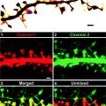 Two-Color STED Imaging of Synapses in Living Brain Slices
 Secondary Ion Mass Spectrometry Imaging of Biological Membranes at High Spatial Resolution
 High Data Output Method for 3-D Correlative Light-Electron Microscopy Using Ultrathin Cryosections
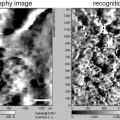 Functional AFM Imaging of Cellular Membranes Using Functionalized Tips
 Nanoimaging Cells Using Soft X-Ray Tomography


Background smoothing of noisy images: Several spatial or time averaging methods are commonly used. Spatial averaging methods, which are based on a spatial low-pass filter including a mean filter, a median filter and a Gaussian filter, remove noise as well as details on the targets to give blurred images. The intensity of target spots is sometimes lost by spatial averaging and a faint spot cannot be distinguished. On the other hand, time averaging, also called moving average or rolling average, averages a series of a certain number of time data to smooth short-term fluctuations such as background noises. Time averaging is likely to have little effect on the intensities of the target spots, because relatively constant values of pixels against time are less affected by the time averaging process. However, time averaging intrinsically involves inevitable effects, especially on the observation of diffusing molecules that are permanently or temporarily confined within some compartments. The effect of time averaging upon changing the exposure time and frame rate has been reported (16). The effect of time averaging is that the position of a molecule appears to be more centralized to the compartments especially when the averaging time is comparable to, or longer than, the time for the target molecules to reach the compartment boundary. In order to reduce such an effect, we process the images using a four-frame exponential moving average with a 2/3 smoothing factor and end this process with spatial averaging of neighboring 3 × 3 pixels. All the averaging processes are performed with ImageJ.
Related posts:
Introduction: Nanoimaging Techniques in Biology
Two-Color STED Imaging of Synapses in Living Brain Slices
Secondary Ion Mass Spectrometry Imaging of Biological Membranes at High Spatial Resolution
High Data Output Method for 3-D Correlative Light-Electron Microscopy Using Ultrathin Cryosections
Functional AFM Imaging of Cellular Membranes Using Functionalized Tips
Nanoimaging Cells Using Soft X-Ray Tomography
Stay updated, free articles. Join our Telegram channel
Full access? Get Clinical Tree
