Fig. 1
a A right-sided disc herniation illustrative model [6]. b Axial view (bottom-up) MRI of a right-sided disc herniation from our data. c Corresponding sagittal view of the herniated disc from our dataset
Disc herniation always occurs in the posterior segment of the disc. The inner gel-like material of the disc, nucleus pulposus, leaks out pressing on a nerve root through a tear in the fibrous wall of the disc, annulus fibrosus [8], as illustrated in Fig. 1, where we show an axial illustrative model and a corresponding clinical MRI (from our dataset) for a right-sided disc herniation with both the axial and sagittal views.
Shape of the posterior segment of the disc, from the sagittal view, is the primary diagnostic tool for the radiologist. The axial view is used for confirmation and for quantification. Working in the sagittal view, our method extracts information of the posterior segment of the disc in a two-step process. First, we use an active shape model to roughly localize a point distribution for the disc body. Then, we have a GVF-snake to delineate the posterior segment of the disc using the outcome of the ASM as its initialization. Because the ASM is a linear model and captures Gaussian point distributions, we add the GVF-snake step to delineate the non-linear shape of the disc posterior segment which is the main technical innovation in this chapter. We validate our method on a clinical dataset of sixty-five cases and achieve over 93 % average classification accuracy.
We also compare our results to the most recent work on disc herniation diagnosis by Alomari et al. [9, 10] that jointly model shape and intensity and we substantially outperform their results. Moreover, our shape-based classifier outperforms the recent work of Michopoulou et al. [11] which is based on an intensity-based classifier. Both recent works test on 33 and 34 cases with an average herniation detection accuracy of 91 and 88 %, respectively. We validate our model on substantially variable dataset of 65 cases and achieve better accuracy over 93 %. Many researchers have proposed methods for the diagnosis of certain vertebral column abnormalities. Bounds et al. [12] utilized a neural network for the diagnosis of back pain and sciatica. Sciatica might be caused by lumbar disc Herniation as well as many other reasons. They have three groups of doctors to perform diagnosis as their validation mechanism. They claimed a better accuracy than the doctors in the diagnosis. However, the lack of data prohibited them from full validation of their system. Similarly, Vaughn [13] conducted a research study on using neural network for assisting orthopedic surgeons in the diagnosis of lower back pain. They classified LBP into three broad clinical categories: Simple Low Back Pain (SLBP), Root Pain (ROOTP), and Abnormal Illness Behavior (AIB) and about 200 cases were collected over the period of 2 years with diagnosis from radiologists. They used 25 features to train the Neural Network (NN) including symptoms clinical assessment results. The NN achieved 99 % of training accuracy and 78.5 % of testing accuracy. This clearly shows training data overfitting.
Tsai et al. [14] used geometrical features (shape, size and location) to diagnose herniation from 3D MRI and CT axial (transverse sections) volumes of the discs. In contrast, we do not presume the availability of the full volume axial view as it is not a clinical standard. They patented their work as a visualization tool for educational purposes. Recently, Michopoulou et al. [11] applied three variations of fuzzy c-means (FCM) to perform atlas-based disc segmentation. Then, they used this segmentation for classification of the disc as either a normal or degenerative disc. They used an intensity-based Bayesian classifier and achieved 86–88 % classification accuracy on 34 cases (five discs each) based on their semi-automatic segmentation of the disc. Similarly, Alomari et al. [9, 10] proposed utilizing a shape and an intensity-based classifier that utilizes an active shape model to extract the shape potentials. However, because the ASM cannot capture the non-linearly shaped posterior segment of the herniated disc, they achieved about 91 % on 33 clinical cases. We extend both these works and present our technical novelty by concentrating on the posterior segment of the disc and capturing that with an additional GVF-snake model on top of the ASM. Furthermore, we reduce the effect of intensity-based information due to the signal intensity inhomogeneity with clinical MRI. We also significantly add variability in the dataset by validating our joint model on 65 clinical cases as opposed to 33 and 34 cases. Furthermore, we achieved an average of 93 % accuracy which substantially outperforms both state-of-the-art results given the dataset size difference.
2 Proposed Method
Our approach has four steps: Disc Localization, Disc Segmentation, Herniation Delineation, and Herniation Classification. This section explains each step:
Disc Localization: The system automatically locates the middle sagittal slice from the MRI volume by index. Then our automatic method starts by a localization step that provides a point inside each disc using the two-level probabilistic model proposed by Corso et al. [15, 16]. Their model labels the set of discs with high level labels 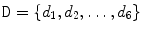 where each
  is the coordinates of the disc point (some point in the disc). They solve the optimization problem:
where  is a set of auxiliary variables, called disc-label variables that are introduced to infer
  from the sagittal image. Each disc-label variable can take a value of
  for non-disc or disc, respectively. The disc-labels make it plausible to separate the disc variables from the image intensities, i.e., the disc-label
  variables capture the local pixel-level intensity models while the disc variables
  capture the high-level geometric and contextual models of the full set of discs. The optimization is solved with a generalized expectation minimization (gEM) algorithm [15, 16]. Figure 2 shows a lumbar sagittal view with labeled discs. Then we obtain a fixed window of
  pixels around each point. This sub-image size is enough to provide the whole disc region for each of the discs connected to the five lumbar vertebrae as shown in Fig. 2.
where each is the coordinates of the disc point (some point in the disc). They solve the optimization problem:(1)
is a set of auxiliary variables, called disc-label variables that are introduced to infer from the sagittal image. Each disc-label variable can take a value of for non-disc or disc, respectively. The disc-labels make it plausible to separate the disc variables from the image intensities, i.e., the disc-label variables capture the local pixel-level intensity models while the disc variables capture the high-level geometric and contextual models of the full set of discs. The optimization is solved with a generalized expectation minimization (gEM) algorithm [15, 16]. Figure 2 shows a lumbar sagittal view with labeled discs. Then we obtain a fixed window of pixels around each point. This sub-image size is enough to provide the whole disc region for each of the discs connected to the five lumbar vertebrae as shown in Fig. 2.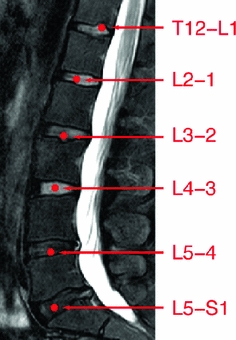
Fig. 3
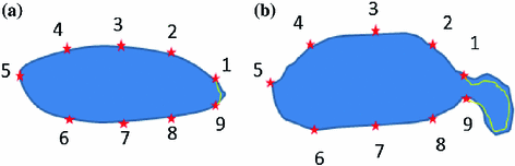
Illustrative model (sagittal view) for a clinically normal disc b herniated disc showing the point distribution ( ) as well as a contour (yellow) that delineates the edge map between points
  and
and  . This figure shows the irregular shape of the normal disc
) as well as a contour (yellow) that delineates the edge map between points and . This figure shows the irregular shape of the normal discDisc Segmentation: We use an active shape model [17] for roughly segmenting the disc body boundary. This step finds the rough shape of the disc body regardless of the herniated (posterior) part. To prepare the training data, we manually select the image slice where herniation is most obvious. Then, we manually mark nine landmark points according to the map shown in Fig. 3. Specifying these landmarks locations is only based on our expertise in the disc segmentation. We name these landmark points from  to
to  . Similar to [17], we initially calculate the mean shape
  where
where  is the size of the training data. Then each disc shape
  , where
  , is recursively aligned to the mean shape
  using generalized Procrustes Analysis to remove translational, rotational, and isotropic scaling from the shape.
to . Similar to [17], we initially calculate the mean shape where is the size of the training data. Then each disc shape , where , is recursively aligned to the mean shape using generalized Procrustes Analysis to remove translational, rotational, and isotropic scaling from the shape.Then, we model the remaining variance around the mean shape with principal components analysis (PCA) to extract the eigenvectors of the covariance matrix associated with 98 % of the remaining point position variance according to the standard method for deriving the ASM’s linear shape representation.
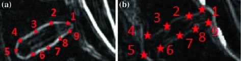
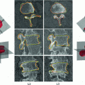
Fig. 4
Feature image result of the range filter  for a Normal disc. b Herniated disc. The ASM point distribution is shown according to the map in Fig. 3
for a Normal disc. b Herniated disc. The ASM point distribution is shown according to the map in Fig. 3 However, we do not use the original MRI image for training the ASM. Rather, we utilize a feature image  that enhances the disc shape by emphasizing the boundaries of the disc and the Thecal Sac (the extension of the spinal canal at the lumbar level [8]). We produce
  by applying a range filter
  on the pixel-wise addition of the normalized co-registered T1- and T2-weighted protocols of the sagittal images
  where
where  and
and  are the normalized T1- and T2-weighted MRI images for the same case. These two images are manually co-registered during the acquisition of the MRI in the clinical standard.
  is the range filter operator where the intensity levels in each
  window are replaced by the range value (maximum – minimum) in that window. This operator
  has high values in abrupt-change regions and small values in smooth regions. Figure 4 shows the features images
  for a normal- and a herniated-disc. The ASM landmark points are also shown in the figure to clarify the ASM land-marking step.
that enhances the disc shape by emphasizing the boundaries of the disc and the Thecal Sac (the extension of the spinal canal at the lumbar level [8]). We produce by applying a range filter on the pixel-wise addition of the normalized co-registered T1- and T2-weighted protocols of the sagittal images where and are the normalized T1- and T2-weighted MRI images for the same case. These two images are manually co-registered during the acquisition of the MRI in the clinical standard. is the range filter operator where the intensity levels in each window are replaced by the range value (maximum – minimum) in that window. This operator has high values in abrupt-change regions and small values in smooth regions. Figure 4 shows the features images for a normal- and a herniated-disc. The ASM landmark points are also shown in the figure to clarify the ASM land-marking step.To apply ASM for detection of the point distribution of the disc body boundary, we apply the mean shape  around the disc point produced by the localization step. Then, we allow the ASM to converge and obtain the boundary.
around the disc point produced by the localization step. Then, we allow the ASM to converge and obtain the boundary.We apply the GVF-snake by initializing its contour (to the line connecting the two points 
 Monitoring of Syndesmophyte Growth in Ankylosing Spondylitis Using Computed Tomography
 Robust Segmentation Framework for Spine Trauma Diagnosis
 Detection and Labelling in Lumbar MR Images
 of Spinal Deformities Using a Parametric Torsion Estimator
 Segmentation and Discrimination of Connected Joint Bones from CT by Multi-atlas Registration
 Morphological and Appearance Features for Predicting Physical Disability from MR Images in Multiple Sclerosis Patients


Related posts:
Robust Segmentation Framework for Spine Trauma Diagnosis
Stay updated, free articles. Join our Telegram channel
Full access? Get Clinical Tree
