billion spent annually on rehabilitation and healthcare. In the past decade there has been a severe shortage of radiologists [2] and projections show that by the year 2020 there will be a significant boom in the ratio of their demand and supply. This concern motivates us to automatically detect and diagnose various lumbar abnormalities from clinical scans to reduce the average time for diagnosis and help to curtail excessive burden on radiologists.
CT and MRI are two popular modalities used to diagnose causes of lower back pain. While on one hand MRI is more expensive, it is non-invasive and also much better in terms of soft tissue detailing. Figure 1 illustrates intervertebral disc herniation diagnosed via the sagittal and axial slices of lumbar MRI. Requirements for CAD systems of the lumbar region are unique since we need to segment the dural sac and/or localize, label and segment the lumbar intervertebral discs before we can diagnose any abnormalities.
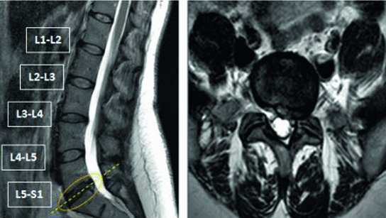
Fig. 1
(Left) Sagittal view of a lumbar MRI showing an L5-S1 disc herniation and (Right) the corresponding axial view of the lumbar MRI confirming a left sided herniation
The lumbar vertebrae are the five vertebrae between the rib cage and the pelvis which are designated L1–L5, starting at the top. The lumbar vertebrae help support the weight of the body and permit movement. The intervertebral discs are fibrocartilaginous cushions serving as the spine’s shock absorbing system, which protect the vertebrae, brain, and other structures. They are named depending on the vertebral bodies above and below, e.g., the disc in between L1 and L2 is named L1-L2 and so on. Dural sac is the membranous sac that encases the spinal cord within the bony structure of the vertebral column as shown in Fig. 2. The human spinal cord extends from the foramen magnum and continues through to the conus medullaris near the second lumbar vertebra, terminating in a fibrous extension known as the filum terminale. The dural sac usually ends at the vertebral level of the second sacral vertebra.
In general, MRI scans are very difficult to segment, since they suffer from partial volume effects and bias fields which might blur the delineation between different kinds of tissues. Moreover, localization of lumbar discs is a challenging problem due to a wide range of variabilities in the size, shape, count and appearance of discs and vertebrae. Similarly accurately segmenting the dural sac is also difficult due to variations in grayscale values and distortion in shape due to various abnormalities like stenosis. To this end we propose an automatic method to simultaneously segment the vertebra, intervertebral discs and the dural sac of clinical sgittal MRI using the neighborhood information of each pixel. In the subsequent sections, we discuss in detail previous research (Sect. 2), our approach (Sect. 3) and experimental results (Sect. 4). Finally we draw our conclusion and discuss the scope for future work in Sect. 5.

Fig. 2
This figure illustrates a cross section of the lumbar vertebrae and spinal cord. The position of the conus medullaris, cauda equina, termination of the dural sac and filum terminale are shown
2 Related Work
There has been quite some research in the direction of automatic dural sac segmentation [9–11], labeling and localization of intervertebral discs [1, 3, 8, 13, 14] and diagnosis of abnormalities [7] from lumbar MRI.
Schmidt et al. [14] introduced a probabilistic inference method using a part-based model that measures the possible locations of the intervertebral discs in full back MRI. They achieve upto 97 % part detection rate on 30 cases. Bhole et al. [3] presented a method for automatic detection of lumbar vertebrae and discs from clinical MRI by combining tissue property and geometric information from T1W sagittal, T2W sagittal and T2W axial modalities. They achieve 98.8 % accuracy for disc labeling on 67 sagittal images. Alomari et al. [1] proposed a two-level probabilistic model that captures both pixel- and object-level features to localize discs. The authors use generalized EM (Expectation Maximization) attaining an accuracy of 89.1 % on 50 test cases. Oktay et al. [13] proposed another approach using PHOG(pyramidal histogram of oriented gradients) based SVM and a probabilistic graphical model and achieved 95 % accuracy on 40 cases. In all these works, the authors have concentrated on localizing the vertebrae and/or intervertebral discs, i.e. they provide a point within the structure. Ghosh et al. [8] presented another approach using heuristics and machine learning methods to provide tight bounding boxes for each disc achieving 99 % localization accuracy on 53 cases.
Koh et al. [10] presented an automatic method for the segmentation of the dural sac using Gradient Vector Flow Field which achieved a similarity index of 0.7 on 52 cases. Horsfield et al. [9] proposed a semi-automatic method for the segmentation of the spinal cord from MRI utilizing an active surface model to assess multiple sclerosis. Koh et al. [11] also proposed an unsupervised and fully automatic method based on an attention model and an active contour model, achieving 0.71 Dice Similarity Index on 60 cases.
3 Proposed Approach
In most of the previous work, segmentation of the dural sac and the intervertebral discs have been handled separately which might lead to overlapping tissue regions. Moreover, some techniques depend on shape models which might lead to errors in case of high variability in appearance. Hence, in our proposed method, we adopt a unified approach where we simultaneously label each pixel as belonging to one of four class labels (vertebra, intervertebral disc, dural sac or background) using a probabilistic atlas and two decision trees based on the neighborhood information of each pixel.
3.1 Our Clinical Dataset
Clinical lumbar MRI used by our group is procured using a 3T Philips MRI scanner at Proscan Imaging Inc. It consists of manually co-registered T2 and T1 weighted sagittal views and T2 weighted axial views. We randomly pick  anonymized cases, all of which have one or more lumbar disc abnormalities. According to the radiologist’s report there are a total of
  herniated discs,
  bulging discs,
  desiccated discs,
  degenerated discs and
  disc levels having mild to severe stenosis.
anonymized cases, all of which have one or more lumbar disc abnormalities. According to the radiologist’s report there are a total of herniated discs, bulging discs, desiccated discs, degenerated discs and disc levels having mild to severe stenosis.For our experiments we use the T2 weighted mid-sagittal slice, each image having a resolution of  . We use our own labeling tool for manual segmentation, which performs B-spline interplolation to interactively give a smooth outline of segmented regions, as shown in Figs. 4b and 5b. We randomly select 40 cases for training and the rest is kept aside for testing.
. We use our own labeling tool for manual segmentation, which performs B-spline interplolation to interactively give a smooth outline of segmented regions, as shown in Figs. 4b and 5b. We randomly select 40 cases for training and the rest is kept aside for testing.Let us denote  as the set of pixel grayscale values in the mid-sagittal image. Our approach treats the segmentation of lumbar MRI as a
  -class problem where each pixel can belong to any one of the following categories:vertebra, intervertebral disc, dural sac and background. The class labels are denoted by the set
  and the set of pixel labels
  where
where  is the output class label for the
  th pixel.
as the set of pixel grayscale values in the mid-sagittal image. Our approach treats the segmentation of lumbar MRI as a -class problem where each pixel can belong to any one of the following categories:vertebra, intervertebral disc, dural sac and background. The class labels are denoted by the set and the set of pixel labels where is the output class label for the th pixel.Fig. 3
Probabilistic Atlas of the lumbar region: a, b and c shows the atlas for the dural sac, the intervertebral discs and the vertebra respectively
3.2 Training Phase
The training phase consists of the following three steps.
3.2.1 Creation of a Probabilistic Atlas
We create a simple probabilistic atlas (probability map) by combining the label information from manual segmentation of the  training images as illustrated in Fig. 3. Since the vetebral column is centrally located in the
  image, we avoid a registration step which can be complicated due to high variability in intensities and shapes of structures in the lumbar region. The atlas is thus a
  matrix where
  and
and  are the total num of rows and columns respectively and
  is the total number of pixels. Thus the probabilistic atlas gives us :
  where
where  is the class label assigned to the
  th pixel and (
 ,
, ) gives the location of the
  th pixel in the image.
training images as illustrated in Fig. 3. Since the vetebral column is centrally located in the image, we avoid a registration step which can be complicated due to high variability in intensities and shapes of structures in the lumbar region. The atlas is thus a matrix where and are the total num of rows and columns respectively and is the total number of pixels. Thus the probabilistic atlas gives us : where is the class label assigned to the th pixel and (,) gives the location of the th pixel in the image.3.2.2 Training a HOG Tree
We train a classification tree [4] based on a pixel’s neighborhood HOG(Histogram of Oriented Gradients) [6]. HOG are feature descriptors popularly used in computer vision and image processing for the purpose of object detection. This technique counts occurrences of gradient orientation in localized portions of an image. For our experiments, given an  w neighborhood around a pixel, we divide it into
  =
=  sub-windows and fix the bin size to
  resulting in a vector of length
  . We empirically fix
  and train the HOG tree using HOG feature vectors and pixel class labels obtained from our
  training images. The hog tree gives us :
 where
where  is the HOG calculated from the
  image neighborhood around the
  th pixel.
w neighborhood around a pixel, we divide it into = sub-windows and fix the bin size to resulting in a vector of length . We empirically fix and train the HOG tree using HOG feature vectors and pixel class labels obtained from our training images. The hog tree gives us : is the HOG calculated from the image neighborhood around the th pixel.3.2.3 Training a Label Tree
Related posts:
 Robust Segmentation Framework for Spine Trauma Diagnosis
Stay updated, free articles. Join our Telegram channel

Full access? Get Clinical Tree


