Fig. 6.1
This figure shows the readout, phase encode, slice select, and radiofrequency (G ro, G pe, G ss, and RF respectively) of a typical Stejskal-Tanner diffusion pulse sequence with an EPI readout. The Stejskal-Tanner core (the diffusion gradients labeled with arrows) is the bipolar gradients, which are separated by a 180° RF pulse. These gradients are dotted to show that they change to vary the amount (amplitude or b-value) and direction of the diffusion sensitivity. The hollow arrows indicate the EPI readout, which in this case is a partial Fourier readout. An EPI readout very efficiently covers k-space and the black RF envelope indicates that the spin echo is designed to occur in the center of k-space (hollow arrow) in the readout
Also note that one can measure the ADC only along the direction of the applied diffusion-encoding gradient. This can be in any direction in the magnet by using a combination of the gradients in the x-, y-, and z-axes. The conventional notation for diffusion direction is the so-called unit vector (i.e., magnitude of the vector equals “1”), in which the tip of the vector points along the direction one wants to measure diffusion. It is important to note that the diffusion section of the pulse sequence (i.e., the diffusion amplitudes on the x, y, and z gradients) is independent from the rest of the pulse sequence, and in fact, a non-diffusion-weighted (b = 0) scan is a part of every diffusion protocol and is simply the diffusion sequence with the diffusion gradient amplitudes set to zero.
For our purposes, the diffusion tensor acquisition can be considered an extension of the Stejskal-Tanner DWI acquisition. The only difference between DWI and DTI is that a DTI acquisition requires a minimum of six or more DWIs, along with at least one image (and often more) without diffusion encoding (i.e., where the diffusion-encoding gradients are turned off, often called a T2w or b = 0 scan) [2, 3]. The acquisition of the set of diffusion images is followed by diffusion post-processing, which is used to calculate the directionality and diffusion coefficient, both of which were covered in more detail in the preceding chapter (Chap. 4). For the purposes of this chapter, note that the six or more diffusion directions required to measure the tensor need to be spread out as much as possible in the 3D sphere of diffusion (D x , D y , D z ). The sphere of diffusion refers to the diffusion direction (direction from the center of the sphere) and the strength of the diffusion-encoding gradients (the distance from the center of the sphere) and directions that are spread evenly around the sphere are mathematically best for the diffusion post-processing and therefore produce the best diffusion tensor results. The minimum of six diffusion directions is required because there are six unknown elements of the diffusion tensor (D xx , D yy , D zz , D xy , D xz , and D yz ).
The groups of diffusion directions (and sometimes multiple diffusion sensitivities, called b-values) are often called “schemes” or “sets.” These sets are often chosen individually for specific applications. One example of these is schemes, often termed High Angular Resolution Diffusion Imaging (HARDI) acquisitions, with generally more than 60 diffusion-encoding directions [4]. A HARDI gradient scheme allows for better differentiation of complex white matter structures and is often used in white matter tract tracing applications. The high spherical resolution allows for observation of directional diffusion differences in highly complex white matter structures such as crossing or fiber bundles with other complex patterns (see Chap. 21 for more details about HARDI techniques). However, regardless of the direction scheme chosen (HARDI or otherwise), the rest of the acquisition (RF pulses, readout method, etc.) is often entirely interchangeable and can be modified to best suit the anatomy and physiology being imaged.
To review, there are two elements essential to Stejskal-Tanner DTI:
Paired diffusion gradients, typically spaced around a 180° RF pulse.
A set of six or more diffusion gradients well spaced around the D x , D y , and D z axes.
Acquisition Background
In order to better describe DTI acquisitions, it is important to understand some of the elements of MRI data acquisition. In this section, we will discuss k-space—the form of the image as it is acquired on the scanner—and complex numbers, both of which are important to keep in mind when discussing the distortions and artifacts typical in DTI acquisitions.
K-Space
The inherent “image” that is acquired by any MRI scanner is not the image that is shown on the scanner. When mapping the acquired MR signal into k-space, it actually becomes the spatial frequency spectrum of the MR image so that a simple Fourier transform (after some processing not discussed here) will yield the MR image and vice versa. In this chapter, we will call the axes in k-space k x and k y for the x- and y-axes respectively. The typical acquisition is a Cartesian—also called a rectilinear or raster—sampling of k-space , which is shown in Fig. 6.2. For typical MR imaging, all the points in k-space are acquired, and then a 2D or 3D Fourier transform is applied to create the 2D or 3D image itself. More details about the transition from k-space to image space—generally called the reconstruction—will be discussed in detail in a later chapter.
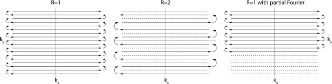
Fig. 6.2
This figure shows the readout in k-space of three bidirectional EPI acquisitions. The different readout direction on odd (arrows going left) and even (arrows going right) lines is the source of EPI “ghosting.” Parallel imaging with a reduction factor of 2 is shown, and for this reduction factor every second line is skipped. Partial Fourier imaging is shown in the third panel. In this case, k-space lines are skipped at the beginning of the readout rather than every other. The acquisition diagram for EPI is shown in Fig. 6.1
Another tricky detail with EPI is that the gradient polarity changes for every other line in k-space, which leads to the well-known “zig-zag” pattern of the EPI readout (Fig. 6.2). While the k y -axis increases linearly for the entire readout, the k-space axis reverses for every other line. Thus, the time axis for every other gradient echo needs to be reversed to match the MR data sample with its location in k-space. If the timing of the odd and even gradient echo lines is off, ghosting artifacts can occur, a phenomenon that will be discussed later.
To review, k-space from an EPI acquisition has three important characteristics:
K-space is the “image” acquired directly from the MRI scanner.
A Fourier transform can be used to convert k-space to an image.
The traversal of k-space may change significantly depending on scan parameters, such as parallel imaging and partial Fourier acquisitions.
Complex Numbers
Each point in k-space, and each point in the image itself is a complex number —even though it is not often shown in the final results. A complex number is a number that consists of both real and imaginary parts—often called magnitude and angle or magnitude and phase in MRI. The phase of the k-space points is important during the image generation, and unwanted phase is the source of most of the image artifacts in EPI.
While the signal magnitude is straightforward for most users to understand because it is simply the strength of the MR signal in each voxel, the concept of having an image where each voxel is a complex number is not as easily understood. An intuitive way to think about it is that if in general the spins in a voxel precess (rotate) slightly faster or slower than normal, by the time the sequence reads out, the angle that is seen is slightly larger or smaller than normal. An analogy to this is a clock that is slightly faster or slower than a perfect clock. If fast, slow, and perfect clocks are set and started at noon, and checked an hour later, the minute hand of the perfect clock will be pointing up at 12 again. However, the minute hand of the slow clock may only be pointing at 50, and the fast clock may be pointing at 5. In this example, the angle (phase) at the time the clock is checked (TE or echo time in MRI) is the angle of the minute hand relative to 12. The phase accrual can be slowed down or sped up deliberately by applying a magnetic field gradient or unintentionally by eddy currents, B 0 inhomogeneities, susceptibility differences, and RF.
The schematic in Fig. 6.3 shows how phase angles change over time with respect to a magnetic field. In fact, phase accrual is the basis for diffusion imaging—the use of the phase coupled with the random walk (diffusion) of spins across very small distances is the indicator that diffusion occurred. The phase is also used in the image acquisition to help form k-space. Many of the artifacts discussed in this chapter are the result of incorrect phase in k-space or image space due to a wide range of factors including motion, diffusion, B 0 inhomogeneities, readout gradient inconsistencies, and others.
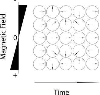
Fig. 6.3
This figure shows the phase or angle in regions of an image with different magnetic fields over time. This phase is often removed from the final images; however this change in phase over time is the source of shim and B 0 artifacts. In some cases, the phase can also affect the combination of data, which can result in cancellation of signal
To review, complex numbers are important in EPI-MRI for two reasons:
All MRI data are complex.
In diffusion processing, the phase is typically discarded at the end of the processing, but it is important to understand because it is the source of many image artifacts in EPI.
The Echo Planar Imaging Acquisition
Echo Planar Imaging
Echo Planar Imaging (EPI) is the clinical and research standard acquisition for DTI. The standard EPI acquisition is usually a single-shot spin-echo acquisition which consists of a 90° excitation, 180° refocusing pulse (Fig. 6.1), and a bidirectional Cartesian readout which linearly traverses k-space (Fig. 6.2) in one go. The EPI trajectory uses a small “blip gradient” to inch its way up the k y -axis, which is orthogonal to the readout. The diffusion-encoding pulses, which are not an inherent part of an EPI readout, are placed on either side of the 180° pulse for Stejskal-Tanner imaging.
The number one reason why the EPI readout is the most popular option for DTI is that any DWI method is notoriously sensitive to motion. This motion sensitivity becomes immediately apparent if one thinks about the minute molecular motion we are trying to capture with this sequence. Any bulk motion while these strong motion-probing gradients are on would pick up substantial phase. Due to the unpredictable nature of bulk motion, these phase changes would most likely differ for each diffusion preparation—readout pair and compete with regular gradient encoding and lead to considerable artifacts. With single-shot EPI the phase errors do not disappear but they are the same for the entire k-space data set and do not bother us. DWI motion sensitivity becomes a problem again when we want to average multiple measurements together. If the number of signal averages is larger than one, the typical method to perform averaging is to directly average the acquired MR signals as they come in. This standard form of MR signal averaging does not work for diffusion images as the individual measurements may interfere destructively (Fig. 6.4). A simple remedy is to reconstruct each acquisition separately and average the magnitude images afterwards. However, averaging in magnitude mode is a challenge in itself. As the noise in MR magnitude data is no longer Gaussian distributed (for the nerds amongst you: it is a Rice-Nakagami distribution), the image becomes hazy in regions with low signal–to–noise ratio (SNR ) as the signal effectively “bounces” off the nonzero mean noise floor. The interested reader is referred to the literature for methods used to resolve this problem [5, 6].
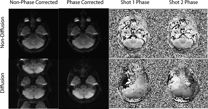
Fig. 6.4
This figure shows an example of a non-corrected and corrected shot combination in non-diffusion and diffusion imaging. Note how the non-diffusion imaging shots have nearly identical phase patterns, and therefore can be combined cleanly—without any noticeable artifacts—even without phase correction. However, because of the sensitivity of diffusion imaging to motion, the diffusion images have phase differences, and it is therefore often impossible to combine the shots without inducing artifacts before phase correction is applied. This case was a two-shot acquisition, so the artifact from poor phase combination largely manifests itself as FOV/2 ghosts, which will be discussed later
With the increasing demand for ever thinner slices, the TR of DTI sequences increases along with the large number of diffusion-encoding directions or intensities for HARDI, Q-ball or q-space imaging. This creates another challenge for diffusion imaging, which is the lengthening of the overall scan time. Single-shot EPI is currently the fastest and most time-efficient diffusion imaging technique, as it is capable of acquiring a whole 2D image in a single excitation and therefore a full DTI dataset in a very short amount of time (Fig. 6.5). Only recently, a further speed-up has emerged through simultaneous multi-band acquisition, but at the time of this writing, this technique is not yet commercially available and is currently only used in research settings [7].
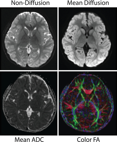
Fig. 6.5
This figure shows DTI results from a medial slice in a “typical” EPI acquisition. It shows the non-diffusion-weighted (b = 0), mean diffusion (b = 1000), mean apparent diffusion coefficient (ADC), and the color FA map. The mean diffusion is simply the average signal intensity from all of the diffusion images acquired. The mean ADC is calculated using the average of the ADC in all three directions (for those of you interested, it is the average of eigenvalues 1–3), and higher values reflect more diffusion in those regions. The color FA indicates the major unidirectional regions of diffusion color coded based on the direction (red is left-right, blue is superior-inferior, and green is anterior-posterior)
In summary, acquiring the entirety of k-space in a single excitation confers two major advantages in DTI. The first is simply the scan efficiency—the speed—of the acquisition. For each slice in DTI, a minimum of seven images—and often many more—must be acquired to fully calculate the diffusion tensor parameters. This is a significant increase in scan time from a single anatomical scan; and by acquiring each image in a single—albeit longer—TR, it allows DTI to remain achievable within a clinical setting. The second advantage of EPI for DTI is the whole image coverage means that it does not require a complicated reconstruction involving data combination in order to prevent phase cancellation between acquisitions. Despite these strengths, and the standard use of EPI in DTI, single-shot EPI is not without its disadvantages, which will be discussed in the following sections.
To review, EPI is used for DWI and DTI for two major reasons:
It is fast because a single image can be acquired for each excitation.
The full image does not require complicated acq uisition and reconstruction tricks to avoid image phase cancellation.
Scan Parameters and Their Effects
In DTI, several scan parameters are changed from standard anatomical imaging in order to work best with the constraints of DTI. A list of the basic parameters, typical values, and comments about them is in Table 6.1. This table is intended as a general guide rather than rules for DTI acquisitions and we hope this will aid your understanding of the parameters and the EPI acquisition.
Table 6.1
Typical DTI parameters
Parameter | Value | Comment |
|---|---|---|
Flip angle | 90° | 90° for the excitation and 180° for the spin echo(es) to achieve maximum signal |
TR | >3 s | At least 2 × T1 of tissue to allow full signal recovery—keep large number of slices within 1 TR by simply increasing TR |
TE | 60–110 ms | As short as possible—depends on maximum gradient strength available for a given b-value as well as whether or not partial Fourier imaging is used |
Partial Fourier | Yes | 20 overscan lines for 128 × 128 |
7/8 partial Fourier | ||
70 % partial Fourier | ||
Go higher on this factor to avoid “worm hole” artifacts. When in doubt use full echo but this increases TE significantly | ||
Matrix size | 128 × 128 | 96–192 are typical, mostly isotropic in plane |
rFOV | 100 % | Cannot do rFOV because PE is along A/P |
Scan % | 100 % | Keep an isotropic in-plane resolution |
FOV | 24 × 24 cm | Large enough to prevent aliasing |
Phase-encode direction | A/P | To keep distortions L/R symmetric on axial scans |
Frequency-encode direction | L/R | |
Parallel imaging factor | 2–3 | Highly dependent on the RF coil |
Some coils afford 4—if reduction factor is too high the parallel imaging noise enhancement impairs image quality | ||
# of b = 0 images | 1–3 | About 1 per 6 diffusion images |
# of diffusion directions | Approx. 21 | 6+ required, more than 100 possible |
Slice thickness | 3 mm | 1–6 mm |
Slice gap | 0 mm | To avoid gaps and better fiber tracking—use interleaved slice acquisition to minimize SNR penalty from slice cross-talk |
b-value | 1000 s/mm2 | 500–5000+ |
For HARDI acquisitions 2500 | ||
For q-space even higher, e.g., 5–8000 | ||
Bandwidth | Maximum for bandwidth | Almost always the maximum (minimum for water-fat shift) possible for the system |
Bandwidth per pixel | ||
Water-fat shift | Minimum for water-fat shift | |
Imaging axis | Axial/Oblique | Axial or oblique close to axial |
Lipid/fat suppression | Yes | SPIR/SPSP/SPAIR/CHESS |
Generally, a DTI acquisition is slower and has more images than anatomical imaging because of the time needed to acquire diffusion-weighted images in at least six directions plus at least a single non-diffusion-weighted (T2w or b = 0) image. It is important to remember that this is the minimum number of images to compute the diffusion tensor. Diffusion acquisitions like HARDI [4] or Q-Ball [8] require many more diffusion directions, sometimes calling for more than 100 diffusion-weighted images per slice. Multiple diffusion magnitudes (b-values) can also be acquired in a single scan [9], as in Q-space imaging. Using more diffusion directions and more b-values can improve the fidelity of the tensor estimation, especially in cases where there are multiple structures within a voxel, such as two tensor tracts crossing or splitting. These methods use more advanced processing methods beyond the standard eigenvalue DTI processing; however a discussion of these methods is beyond the scope of this chapter.
A side effect of acquiring many diffusion directions and b-values is that the many acquisitions act as a form of averaging, which increases the signal–to–noise–ratio (SNR) of the diffusion tensor images (Fig. 6.6). This is advantageous because another consideration is that the reduction of the MR signal due to diffusion weighting causes the SNR to be generally lower in the diffusion-weighted images when compared to an anatomical image with similar scan parameters. In clinical practice, acquiring more diffusion directions rather than repeating diffusion directions is the preferred method of performing averaging. This is done because it is a robust way to both increase the SNR and ensure more than enough diffusion directions were acquired.
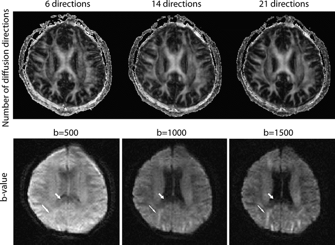
Fig. 6.6
This figure shows images with different numbers of diffusion directions used (top row) as well as different b-values used (bottom row). The top row shows the fractional anisotropy maps (brighter indicates more directionality in the tissue) all with a b-value of 1000, calculated using 6, 14, and 21 directions from left to right. Note that even though nothing else is changed between the acquisitions, the clarity of the images improves as more diffusion directions are added, which is primarily due to the averaging effects of more images. The bottom row shows (in a separate slice) a single diffusion direction (applied left-right) with b-values of 500, 1000, and 1500 s/mm. Note that the signal is higher in the b = 500 s/mm scan, but it is difficult to differentiate between structures. Also note that depending on the direction of the fiber tract, higher b-values tend to emphasize (thin arrow) or de-emphasize (thick arrow) the structures
Furthermore, as the b-value increases, the SNR in the individual diffusion images decreases (Fig. 6.6). This becomes a trade-off between the contrast between the diffusion-weighted images and their SNR; the former potentially showing more detail and the latter providing less-noisy images. A simple solution to counteract the lower SNR is to increase the voxel size compared to that used with anatomical imaging.
Another consideration of increased b-values is increased eddy current distortions, which are covered in detail later in this chapter. In short, higher b-values—stronger diffusion gradients—can cause distortions in the image. These may not be obvious by looking at the images, but they may cause artifacts around the edge of the brain in the processed maps.
The first general MRI scan parameter to discuss is the echo time (TE). With the inclusion of the diffusion-encoding gradients, the minimum TE is increased by the duration of the gradients. While the minimum TE—or very close to the minimum—is often used, the minimum TE is often far longer than what is possible without the diffusion gradients, as in the non-diffusion-weighted image. The one caveat for the TE is that it should be the same for all diffusion directions and weightings, including the non-diffusion-weighted image, in order to prevent any T2 decay (or differences thereof) from influencing the calculation of the diffusion coefficient. A standard TE for DTI is around 80 ms, although it can vary greatly depending on the scanner’s gradient hardware as well as the requested scan and diffusion parameters.
The increased TE is also a source of decreased SNR relative to anatomical MRI. In conjunction with the diffusion-encoding gradients, which also decrease the signal, DTI acquisitions have a lower SNR than anatomical images. It is in part because of the low signal that often more than 15 diffusion-encoding directions and multiple T2-weighted images are used in standard clinical DTI.
Note that unlike in anatomical imaging where a long TE generates T2-weighted contrast in the image, the ADC images only have diffusion contrast. While the individual images in the series have T2-weighted contrast from the TE, this contrast is removed in the DTI processing because all of the diffusion images have the same TE. This results in images which are unaffected by image contrast beyond that intentionally created by the diffusion gradients.
Because of the increased TE, the minimum repetition time (TR) is also increased. An important point to remember for DTI is that the TR should be at least three times the tissue T1-relaxation time in order to allow near full relaxation of the spins. In the brain, this means that the minimum TR is considered to be at least 3 s, and preferably more than 5 s. Often, however, with multi-slice scans, the time it takes to acquire all of the slices—and make it fit into one TR—is more than the 3, or even 5-s minimum. While a TR that is too low reduces the SNR and can induce T1-weighting into the diffusion images, anything beyond approximately 5 s does not improve or degrade the images in any way.
Another important scan parameter is the resolution of the scan. EPI-DTI is typically acquired at a relatively low resolution compared to anatomical imaging protocols that take approximately the same amount of time. The low resolution is primarily because of the reduced signal in the diffusion-weighted images caused by the diffusion-encoding gradients, as well as the time required to encode the seven or more diffusion-encoding directions, which are required for a sufficient SNR for the tensor calculation.
Typically, the resolution is as high as possible while still allowing a high enough SNR as is required by the application. The balance between resolution, SNR, and the number of diffusion-encoding directions in general is an open research question, and even for specific applications it is not easy to determine without specific testing. It often depends on the anatomy under exploration, as well as the SNR and resolution that the post-processing methods require. Because of these complicated trade-offs, it is important to check previous protocols and work to verify what is required of the technique and to confirm that it is possible with your scanner before scanning patients.
To review, there are three major parameters that are treated differently for DTI than most other MRI scans:
The TE is set as short as possible to get the highest SNR possible because the contrast is created with the diffusion gradients, not the TE and TR.
The TR is set to be as short as possible for speed, but it must stay longer than three times the expected T1 of the tissue—typically more than 3 s.
The resolution is set as high as possible while still allowing for good SNR. There is no equation for this; it is all determined by testing.
Consequences of the EPI Trajectory
This section will discuss the EPI trajectory and common artifacts, which are often seen in conjunction with DTI-EPI. The EPI trajectory is unique because it samples multiple Cartesian lines in k-space in a single readout. This is very efficient in terms of scan time and has the nice property for diffusion-weighted imaging that the whole image can be acquired in a single excitation, which helps prevent problems from diffusion-encoding induced phase errors which will be discussed later.
However, acquiring data in a single, long readout enhances several types of artifacts, which can pose problems when reading or analyzing the images. These consist of:
Chemical shift artifacts in which fat/lipid signal is also shifted significantly relative to the rest of the image and can cause masking of the true image in places of overlap.
Distortions due to off-resonance in the object from main magnetic field distortions such as B 0 inhomogeneities or a bad shim.
Ghosting, which is due to inconsistent phase encoding in odd and even lines in k-space.
The main consequence of a Cartesian EPI readout with the phase-encode lines acquired linearly from one edge of k-space to the other is that the EPI readout is very fast in the readout direction (k x ), but very slow in the phase-encode direction (k y ) (Fig. 6.2). The consequence of this readout is that artifacts, which in other scan types manifest in the readout direction, present very strongly in the phase-encode direction in EPI. For example, the fat-water shift can be tens of pixels in the phase-encode direction in EPI images, whereas in normal gradient or spin-echo imaging, the shift is typically less than two pixels in the readout direction. Do note that different vendors report either bandwidth in kHz (GE), bandwidth in Hz per pixel (Siemens), or water-fat shift (Philips).
This water-fat shift is caused by the different resonant frequency of fat compared to water. As mentioned above, the slow read progression in k y causes the chemical shift artifact as in standard gradient or spin-echo imaging. However, chemical shift is not limited to chemical species; the same principle applies to any region where off-resonance is present. In EPI images this causes the signal from the off-resonance regions to be shifted, which—due to the gradual off-resonance change—looks like stretching or signal pileup in the image rather than a distinct shift (Fig. 6.7). This can be caused by off-resonance effects such as a poor shim, or more commonly by air-tissue interfaces such as those adjacent to the sinuses or other cavities in the head, which cause irregular magnetic fields in the neighboring brain tissue.
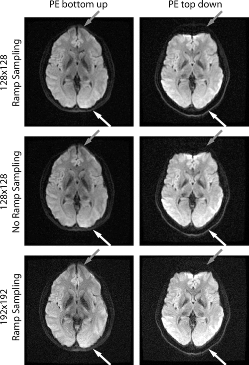
Fig. 6.7
These EPI images show off-resonance induced artifacts due to an inhomogeneous magnetic field. When comparing the phase encode (PE) up vs. down, it is clear that the image is either stretched or compressed in regions with off-resonance, such as the regions indicated by the gray and white arrows. Even though this artifact affects the whole image, the gray and white arrows show regions where the differences between the up and down PE artifact are easy to see. The speed at which the image is acquired decreases from the fastest, (a matrix of) 128 × 128, to 128 × 128 without ramp sampling, to the slowest, 192 × 192. Because of this reduction in the sampling speed, the artifacts increase, which is easy to see when comparing regions near the gray or white arrows for the three different sampling speeds. Note that decreasing the resolution is not the only way to increase the sampling speed and therefore decrease the off-resonance artifacts; however it is a way to modulate the distortion
The B 0 (main magnetic field) and chemical shift artifacts are caused by off-resonance differences or natural chemical frequency in different regions of the image. These artifacts can be reduced with careful shimming and fast scans, and fat saturation pulses respectively. In fact, because the resonance frequency of fat is not the same as water, fat is typically shifted a significant amount when compared to the rest of the image, often into the brain itself (Fig. 6.8). Lipids have a very low diffusion coefficient and therefore voxels that have fat overlaid appear hypointense (dark) on ADC maps. Similarly, residual lipid ghost often confounds diffusion anisotropy maps. Because of this, a fat saturation pulse, or some other method of suppressing the fat signal, is required. Alternatively, one can use “water-only” excitation pulses (i.e., spectral-spatial RF pulses) that do not excite fat protons within a slice.
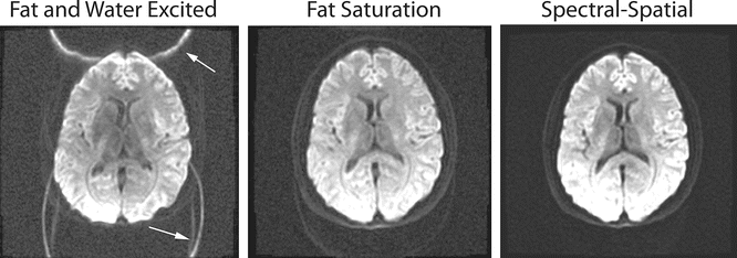
Fig. 6.8
Lipid suppression is very important in EPI and DTI imaging in order to remove the unwanted fat signal from the diffusion calculations. The first image, in which both fat and water are excited with a normal RF pulse, shows how the fat signal is shifted and can disrupt regions in the image. The next two images show how both fat saturation and spectral-spatial pulses work well to suppress the unwanted fat signal
Another artifact called “ghostin g” is inherent to EPI in which the k-space readout is performed in both directions, which is what is shown in Fig. 6.2. This is the most common type of EPI used in the clinic. Ghosting is caused by differences between odd and even (readouts progressing to the right and left respectively) k-space lines. These differences manifest as image “ghosts” at a fraction of the field of view. For single-shot EPI, with altering odd and even echoes, the ghost is shifted by half the FOV. Ghost artifacts like this (called FOV/2 ghosts) are often fixed in the reconstruction, though this is not always the case and ghosting may be more prevalent if the imaging plane is oblique. Similar to residual fat overlaying on the tissue of interest, the diffusion tensor information can be confounded by the aliased FOV/2-ghost. Quantitative measurements as well as scalar images (e.g., b = 0) will be most corrupted when there is a substantial signal intensity difference between the original and the aliased voxel (e.g., brain tissue vs. eyeball).
There are two different causes of ghosting: the phase difference and shift between the even and odd echoes in k-space. Both of these result in ghosting, but their appearance is different and they are caused by the intercept and slope of the phase terms, respectively [6]. Figure 6.9 shows different types of ghosting, and disabling ghost correction as seen in Fig. 6.10 shows combinations of both echo phase and echo shift ghosts.
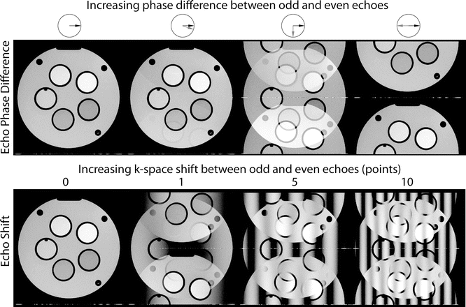
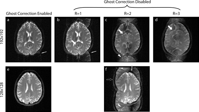
Fig. 6.9
This figure shows how differences between odd and even echoes cause EPI ghosting. The first row shows how the phase difference between the echoes causes varying intensity ghosts in the image. Note how (from left to right) the 0° (no ghosting) and 18° vary only slightly, but at 90° the ghost and original have equal intensities, and at 180° only the aliased image remains visible. The arrows in the circles above the first row show the phase of the even echo and odd echo in black and gray respectively. The second row shows how shifts between the odd and even echoes cause bands of aliased and un-aliased regions in the image. Note that (from left to right) the number of ghosted bands is equivalent to an increased echo shift in k-space. For all these images the phase-encode direction is up-down
Fig. 6.10
These images show EPI ghosting with different parallel imaging factors. Note that with the exception of (a, e) these images were generated by turning off the “ghost correction” portion of the reconstruction, ghosting can also arise when the ghost correction is used, but is simply unsuccessful. This is the case in the 192 × 192 resolution ghost corrected image (a, white arrow) where some slight aliasing is still present, which is similar to that in (b). The “ghosts” are shifted by a fraction related to the parallel imaging used and are caused by inconsistent even and odd readout lines (see Fig. 6.2). Traditional EPI ghosts (also called N/2 or Nyquist ghosts) are shifted halfway around the image like in (b), i.e., FOV/2. However, when parallel imaging is used, the ghost shift changes relative to the parallel imaging factor: FOV/(2R) where R is the parallel imaging acceleration. The thick arrows show the top of a “ghosted” brain in the R = 1, 2, and 3 images (b–d), which shows how it shifts with the changes in the parallel imaging factor. The two images for a parallel imaging acceleration of 2 show how different ghosting can look between similar images. The gray arrow in (f) shows a vertical band where no correction is needed to produce a good image; however in the same image, the hollow arrow shows a band where the image is entirely ghosted and the true image (e) is not represented
Another variant of magnetic field distortions is due to eddy currents (see section “Examples and Mitigation of DTI-EPI Artifacts”) induced in the conducting elements of the magnet by switching the strong diffusion-encoding gradients and which cause spatiotemporal variations of the effective field “seen” by the protons.
To review, there are three common types of artifacts which can manifest—typically, but not always—in the phase-encode direction:
Hardware Limitations
There are many hardware limitations in MRI that are considerations for DTI; some of which are imposed by engineering challenges, and some by the human body itself. There are two major limitations when it comes to the performance of the magnetic field gradients and one for the use of the radiofrequency (RF) system.
For the gradient systems, which are especially stressed during DTI acquisitions due to the extremely strong diffusion gradients, the two major limitations are the maximum gradient strength and the rate at which the gradient changes strength (slew rate). Table 6.2 lists several scan parameters that can affect the gradient system and influence the maximum gradient strength and slew rate in some way.
Table 6.2


Scan parameter and gradient limitations
Related posts:

Stay updated, free articles. Join our Telegram channel
Full access? Get Clinical Tree
