Symptomatic Versus Asymptomatique Plaque Classification in Carotid Ultrasound

Fig. 29.1

Block diagram of the proposed technique; the blocks outside the dotted shaded rectangular box represent the flow in the off-line system, and the blocks within the dotted box indicate the online system

2.2 Data Acquisition and Preprocessing

We used 150 asymptomatic and 196 symptomatic (a total of 346) carotid plaque ultrasound images in this work. These images were collected from patients referred to the Vascular Screening Diagnostic Center, Nicosia, Cyprus, for diagnostic carotid ultrasound to detect both presence and severity of internal carotid stenosis. Approval from Institutional Review Board and consent from patients were obtained prior to conducting the study. Subjects with cardioembolic symptoms or distant symptoms (>6 months) were not included in this work. The plaques with less than 50% stenosis were not included in the database [5]. We also excluded plaques from emergency cases scanned after normal working hours as the scanning was often performed by personnel not trained in plaque image capture. The ultrasonographers who conducted the examinations and obtained the plaque images knew the reason for referral, as they performed routine diagnostic testing for the presence and grading of stenosis. However, for the purpose of studies such as the present, the database images were anonymized and the persons who subsequently did the image normalization and image analysis did not know whether the plaques were symptomatic or asymptomatic [10].

The following prerequisites essential for successful image normalization were carried out: (1) Dynamic range adoption. (2) Frame averaging (persistence). (3) Time gain compensation curve (TGC) was sloping through the tissues was positioned vertically through the lumen of the vessel because the ultrasound beam was not attenuated when passed through blood. This ensured that the adventitia of the anterior and posterior walls had similar brightness. (4) Gain adjustment. (5) Postprocessing with a linear transfer curve. (6) The ultrasound beam was at 90° to the arterial wall. (7) The minimum depth was used so that the plaque occupied a large part of the image. (8) The probe was adjusted so that Adventitia adjacent to the plaque was clearly visible as a hyperechoic band which may be used for normalization. The grayscale images were normalized (using blood and adventitia as reference points) manually by adjusting the image linearly so that the median gray level value of blood was in the range of 0–5, and the median gray level of adventitia (artery wall) was in the range of 180–190.

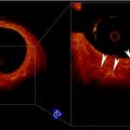
The plaques from patients having retinal or hemispheric symptoms (unstable plaques), such as stroke, Transient Ischemic Attack (TIA), and Amaurosis Fugax (AF), were grouped as symptomatic plaques (88 stroke, 70 TIA, and 38 AF) ~196. Asymptomatic plaques were from patients who had no symptoms in the past. During preprocessing, the Region of Interest (ROI) was selected by medical practitioner from each of the studied images prior to feature extraction. The vascular surgeons and sonographers are trained to identify the hypoechoic region representing hard plaque or stenosis. Therefore, we adapted the manually segmented plaque regions in this work. The nature of the disease is focused on the vessel wall that specifically changes the morphology of the lumen-intima interface from slow gradual lipid formation and maturing into hard plaque or loose island of hemorrhage [11]. Thus, the young and old plaques are all focused towards the vessel disease which yields the information in the form of echogenicity in the ultrasound image [10]. Therefore, the focused ROI constitutes <25% of the image frame, and hence, the vascular surgeons are keenly interested in characterization of plaque in this regional information. We, therefore, focused on analyzing this small ROI traced by the vascular surgeon. Typical symptomatic and asymptomatic carotid images are shown in Fig. 29.2a, b. Figure 29.3a, b shows the ROIs of symptomatic and asymptomatic carotid images.

Fig. 29.2

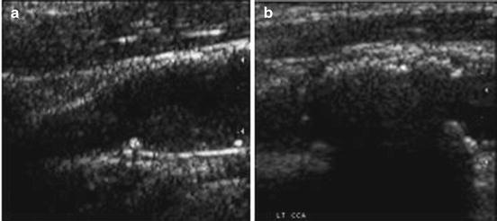
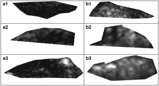
Carotid images: (a) symptomatic (AF) and (b) asymptomatic (AS). Source: [12], ^© IEEE, 2012

Fig. 29.3

Region of interest extracted from the carotid plaque ultrasound images of (a) symptomatic (AF) and (b) asymptomatic (AS) patients. Source: [12], ^© IEEE, 2012

2.3 Feature Extraction

In this work, we used two-dimensional (2D) DWT and averaging algorithms for feature extraction. The DWT transform of a signal x is determined by sending the signal through a sequence of down-sampling high and low pass filters. The low pass filter is defined by the transfer function g[n] and the high pass filter by h[n]. The output of the high pass filter D[n], known as the detail coefficients, is obtained as follows:

$D[n]=\sum\limits_{{k=-\infty}}^{\infty } {x[k]h[2n-k]}$

(29.1)

The output of the low pass filter, known as the approximation coefficients, is found by using the following equation.

$A[n]=\sum\limits_{{k=-\infty}}^{\infty } {x[k]g[2n-k]}$

(29.2)

The frequency resolution is further increased by cascading the two basic filter operations. To be specific, the output of the first level low pass filter is fed into the same low and high pass filter combination. The detailed coefficients are output at each level, and they form the level coefficients. In general, each level halves the sample number and doubles the frequency resolution. Consequently, in the final level, both detail and approximation coefficients are obtained as level coefficients. For 2D signals, the 2D DWT can be used. We used wavelet packet decomposition (WPD) for images. These images are represented as an m × n grayscale matrix I[i, j] where each element of the matrix represents the intensity of 1 pixel. All non-border pixels in I[i, j], where $i\notin \{0,m\}$ and $j\notin \{0,n\}$ , have eight immediate neighboring pixels. These eight neighbors can be used to traverse through the matrix. However, changing the direction with which the matrix is traversed just inverts the sequence of pixels, and the 2D DWT coefficients are the same. For example, the WPD result is the same when the matrix is traversed from left to right as from right to left. Therefore, we are left with four possible directions, which are known as decomposition corresponding to 0° (horizontal, Dh), 90° (vertical, Dv), and 45° or 135° (diagonal, Dd) orientations. The implementation of this algorithm follows the block diagram shown in Fig. 29.4. The diagram shows the N × M dimensional input image I[i, j] and the results for level 1. In this work, we found that the results from level 1 were sufficient to obtain significant features.

Fig. 29.4

Discrete wavelet transform (DWT) decomposition. Source: [12], ^© IEEE, 2012

In this work, we evaluated several wavelet functions. Each of these wavelet functions has both a unique low pass filter transfer function g[n] and a unique high pass filter transfer function h[n]. Figure 29.5 shows the transfer functions for the Biorthogonal 3.1 (bior3.1) family used in this work.

Fig. 29.5

Transfer functions of the Biorthogonal 3.1 wavelet (bior3.1). Source: [12], ^© IEEE, 2012

The first level 2D DWT yields four result matrices, namely Dh ₁, Dv ₁, Dd ₁, and A ₁, whose elements are intensity values. Figure 29.6 shows a schematic representation of these result matrixes. Unfortunately, these matrixes cannot be used for classification directly, because the number of elements is too high. Therefore, we defined two averaging methods that represent result matrixes with just one number. The first method is used to extract average measures from 2D DWT result vectors.

Fig. 29.6

Wavelet-based image decomposition. Source: [12], ^© IEEE, 2012

$$$ \mathrm{Average}\,D{h_1}(Ah)=\frac{1}{{N\times M}}\sum\limits_{x=<N> } {\sum\limits_{y=<M> } {\left| {D{h_1}(x,y)} \right|} } $$ ” src=”/wp-content/uploads/2016/08/A271459_1_En_29_Chapter_Equ00293.gif”></DIV></DIV><br /> <DIV class=EquationNumber>(29.3)</DIV></DIV><br /> <DIV id=Equ00294 class=Equation><br /> <DIV class=EquationContent><br /> <DIV class=MediaObject><IMG alt=$ } {\sum\limits_{y= } {\left| {D{v_1}(x,y)} \right|} } $$ ” src=”/wp-content/uploads/2016/08/A271459_1_En_29_Chapter_Equ00294.gif”>

(29.4)

The final averaging method uses averages not the intensity values as such but the energy of the intensity values.

$$$ \mathrm{Energy}\;(E)=\frac{1}{{{N^2}\times {M^2}}}\sum\limits_{x=<N> } {\sum\limits_{y=<M> } {{{{(D{v_1}(x,y))}}^2}} } $$ ” src=”/wp-content/uploads/2016/08/A271459_1_En_29_Chapter_Equ00295.gif”></DIV></DIV><br /> <DIV class=EquationNumber>(29.5)</DIV></DIV></DIV><br /> <DIV class=Para>These three elements form the feature vector.</DIV></DIV><br /> <DIV id=Sec00296 class=$

2.4 Feature Selection

We have used t-test [13] to verify if the features are significant enough to be able to accurately discriminate the symptomatic and asymptomatic classes. In this test, initially, the null hypothesis is assumed that the means of the feature from the two classes are equal. Then, the t-statistic, which is the ratio of difference between the means of a feature from two classes to the standard error between class means, and the corresponding p-value are calculated. The p-value is the probability of rejecting the null hypothesis given that the null hypothesis is true. In our case, we assumed a normal distribution of the features, but the scaling term in the test statistic was known. Therefore, it was replaced by an estimate based on the data. A low p-value (<0.01 or 0.05) indicates that the means are significantly different for the two classes, and hence, the feature is significant.

2.5 Classification

SVM is a hyperplane-based nonparametric classifier. When it is trained using input features–output ground truth class label pairs, it outputs a decision function which can be used to test new input features. Assuming that the class label c = −1 for asymptomatic class and +1 for symptomatic class, the SVM algorithm maps the training set into a feature space and attempts to locate in that space a hyperplane that separates the positive from the negative examples. During the testing of a new unlabeled image, the algorithm maps the image’s feature vector into the same feature space and determines the class based on which side of the separating plane the vector is present. Thus, the main objective of SVM is to determine a separating hyperplane that maximizes the margin between the input data classes that are plotted in the feature space [14–16]. In order to determine the margin, two parallel hyperplanes are constructed, one on each side of the separating hyperplane with the help of the training data. Consider two-class classification using a linear model of the form

$y(x)={w^{\mathrm{T}}}\phi (x)+b$

(29.6)

where $\phi (\cdot )$ denotes the feature transformation kernel, b is the bias parameter, and w is the normal to the hyperplane. The training data consists of the input feature vectors x and the corresponding classes c. c = −1 for asymptomatic class and +1 for symptomatic class. During the testing phase, the new feature vector is classified based on the sign of y. The perpendicular distance to the closest point from the training data set is the margin, and the objective of training an SVM classifier is to determine the maximum margin hyperplane and also to assign a soft penalty to the samples that are on the wrong side of the margin. Support vectors are those points that the margin pushes up against. The problem becomes an optimization problem where we have to minimize

$\begin{gathered} C\sum\limits_{i=1}^N {{\xi_i}+\frac{1}{2}{{{\left\| w \right\|}}^2}} \hfill \\ {c_i}y({x_i})\geq 1-{\xi_i},\quad \xi \geq 0 \hfill \\ \end{gathered}$

(29.7)

where ξ _iare the penalty terms for samples that are misclassified, and C is the regularization parameter which controls the tradeoff between the misclassified samples and the margin. The first term in (29.7) is equivalent to maximizing the margin. This quadratic programming problem can be solved by introducing Lagrange multipliers a _nfor each of the constraints and solving the dual formulation. The Lagrangian is given by

$\begin{array}{lll} L(w,b,a)&=\frac{1}{2}{{\left\| w \right\|}^2}+C\sum\limits_{i=1}^N {{\xi_i}}\hfill\\ & \quad -\sum\limits_{i=1}^N {{a_i}[{c_i}y({x_i})-1+{\xi_i}]} -\sum\limits_{i=1}^N {{\mu_i}{\xi_i}} \end{array}$