be an Euclidean or digital space (i.e.  or
or  with
with  ). Let
  be a subset of
  . Let
. Let  denote the class of all subsets of
  :
:  . Let
. Let  denote the complement of
  , i.e. the set of all points of
  that do not belong to
  :
:  . Let
. Let  denote the reflection of
  , i.e. the set
  transformed by a central symmetry:
  . Finally, we will denote by
  the translate of
  by
by  defined by
  .
.
The basic operators of erosion and dilation of  by the Structuring Element (SE)
  are written respectively
  and
and  . They are defined using the Minkowski subtraction (
 ) and addition (
 ):
):


 by the Structuring Element (SE)
  are written respectively
  and
and  . They are defined using the Minkowski subtraction (
 ) and addition (
 ):
):
(1)

(2)
2.2 Binary HMT
Being given a subset  of
of  , the principle of the HMT is to look for all positions
  in
in  where a structuring element
  called the foreground fits in the shape (
 ) while another structuring element
  called the background fits in the complement of
  (
( ). The HMT of
  by the structuring elements
  , noted
  , can be defined in terms of Minkowski subtraction and addition (structuring erosion and dilation):

A direct consequence of this definition is that if  and
and  have a non-empty intersection, then
  is empty for all
  in
in  (a given pixel cannot simultaneously belongs to the foreground and to the background). One can also note that: first, the second formulation of (Eq. 3) is known as the interval operator from [15] and second, the complementation does not appear in the last formulation which allows to naturally extend the HMT to gray-level images where complementation is not defined.
 of
of  , the principle of the HMT is to look for all positions
  in
in  where a structuring element
  called the foreground fits in the shape (
 ) while another structuring element
  called the background fits in the complement of
  (
( ). The HMT of
  by the structuring elements
  , noted
  , can be defined in terms of Minkowski subtraction and addition (structuring erosion and dilation):
(3)
 and
and  have a non-empty intersection, then
  is empty for all
  in
in  (a given pixel cannot simultaneously belongs to the foreground and to the background). One can also note that: first, the second formulation of (Eq. 3) is known as the interval operator from [15] and second, the complementation does not appear in the last formulation which allows to naturally extend the HMT to gray-level images where complementation is not defined.
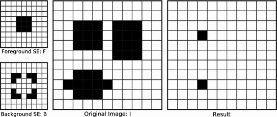
Figure 1 illustrates the application of the hit-or-miss transform on a binary image. Our goal here is to detect  squares with possible extensions along edges. It is noteworthy that the two structuring elements do not need to cover the whole neighborhood of a pixel and some pixels, as the middle of the edges of the square, can be excluded from the decision process by neither putting them in
  nor in
  . This is a first attempt to ensure robustness to uncertainty or noise. Some more advanced solutions, not specific to binary images will be reviewed in Sec. 5.
 squares with possible extensions along edges. It is noteworthy that the two structuring elements do not need to cover the whole neighborhood of a pixel and some pixels, as the middle of the edges of the square, can be excluded from the decision process by neither putting them in
  nor in
  . This is a first attempt to ensure robustness to uncertainty or noise. Some more advanced solutions, not specific to binary images will be reviewed in Sec. 5.
Fig. 1
Example of application of binary HMT to detect 3 x 3 squares with possible extensions along edges [27]. The pixels belonging to the images are in black while those belonging to the complement are in white. The top left image represents the foreground SE:  , origin of the image is at the centre of the square. The bottom left image is the background SE
  , with same origin as
  . The middle image is the original image
  . And the right image is the result of the HMT applied on
  with SEs
  and
and 
 , origin of the image is at the centre of the square. The bottom left image is the background SE
  , with same origin as
  . The middle image is the original image
  . And the right image is the result of the HMT applied on
  with SEs
  and
and 
3 Template Matching in Grayscale Images
We recall here basics of Mathematical Morphology in the grayscale case, with adequate definitions and notations. The various definitions of the HMT on grayscale images (e.g.,[8, 23, 31, 34]) will then be presented and discussed, with comprehensive examples.
3.1 Grayscale Mathematical Morphology
We now consider the case of grayscale images, i.e.of mappings from  to the set of values
  (
( ). Moreover, we assume that
  is a complete lattice, i.e. a non empty set equipped with a partial ordering
  , an infimum
  and a supremum
  such that the infimum and supremum of any non empty subset of
  belongs to
  (for all
  ,
,  and
and  ). The lattice
  is thus bounded by its least element
  and its greatest element
  . For grayscale images we usually take
  or
or  . The notion of structuring element naturally extends to the one of structuring function (SF) which is simply an element of
  .
.
 to the set of values
  (
( ). Moreover, we assume that
  is a complete lattice, i.e. a non empty set equipped with a partial ordering
  , an infimum
  and a supremum
  such that the infimum and supremum of any non empty subset of
  belongs to
  (for all
  ,
,  and
and  ). The lattice
  is thus bounded by its least element
  and its greatest element
  . For grayscale images we usually take
  or
or  . The notion of structuring element naturally extends to the one of structuring function (SF) which is simply an element of
  .
.The definitions of the binary erosion (Eq. 1) and binary dilation (Eq. 2) then naturally extend to grayscale images. Let  in
in  be a grayscale image and
  in
in  be a structuring function. The grayscale erosion
  and dilation
  of
of  by
by  are then defined for all
  by:
by:


where  is the support of
  , i.e.the set of points of
  where
where  is greater than the least element
  :
:  . These formulas can lead to disinclination like
  plus
plus  . To keep consistency
  plus
plus  must be valued as
  in Eq. 5 and as
  in Eq. 4.
 in
in  be a grayscale image and
  in
in  be a structuring function. The grayscale erosion
  and dilation
  of
of  by
by  are then defined for all
  by:
by:
(4)

(5)
 is the support of
  , i.e.the set of points of
  where
where  is greater than the least element
  :
:  . These formulas can lead to disinclination like
  plus
plus  . To keep consistency
  plus
plus  must be valued as
  in Eq. 5 and as
  in Eq. 4.
3.2 Grayscale HMT
The binary HMT was first extended to grayscale images by Ronse [31] and then many other definitions followed: by Shaefer [32], Khosravi [18], Raducanu [29], Soille [36], Barat [7], Perret [27]. A recent survey on grayscale HMT is given in [22]. These various definitions have been recently unified into a common theoretical framework for graylevel interval operators [23]. In the binary case, the interval operator (second line of Eq. 3) looks for each translation  if the image fits between the background SE translated at
  and the complement of the background SE also translated at
  . In the grayscale case, the sought template is translated not only horizontally (by a point
  ), but vertically as well (by a finite graylevel
  ) in an attempt to detect the positions where it fits (Fig. 2). Specifically, we will note
  the translation of
  by a couple
  : for all
  ,
,  .
.
 if the image fits between the background SE translated at
  and the complement of the background SE also translated at
  . In the grayscale case, the sought template is translated not only horizontally (by a point
  ), but vertically as well (by a finite graylevel
  ) in an attempt to detect the positions where it fits (Fig. 2). Specifically, we will note
  the translation of
  by a couple
  : for all
  ,
,  .
.According to the unified theory for grayscale HMT [23], a grayscale HMT is decomposed into two stages:
Let us observe that in the binary case, the fitted pixels are the ones retained by the HMT, and their valuation is simply equal to one (or foreground).
the fitting, where the locations fitting the given structuring functions, describing the sought template, are computed,
and valuation, where the resulting image containing the previously detected locations is constructed.
3.2.1 Fitting
We first describe the different fittings. Let  be a grayscale image and
  be a couple of structuring functions describing the sought template such that
  . Formally a fitting is a mapping from
  into
into  where
where  can be a subset of
  or any set of values. A first fitting involved in Ronse’s HMT is given by:


where  , is the dual of
  .
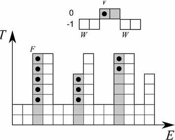
.  is thus the set of all translations where the image lies between both structuring functions (Fig. 3).
 be a grayscale image and
  be a couple of structuring functions describing the sought template such that
  . Formally a fitting is a mapping from
  into
into  where
where  can be a subset of
  or any set of values. A first fitting involved in Ronse’s HMT is given by:
(6)

(7)
 , is the dual of
  .
.  is thus the set of all translations where the image lies between both structuring functions (Fig. 3).
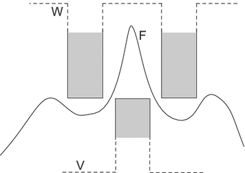
Fig. 3
Illustration of  (Eq. (6)). We consider a function
  from
from  into
into  and the two structuring functions
  and
and  (the origin is on the left pixel of
  ). The result of
  is the set of points of
  marked by a black circle inside
  . We also give the result of the application of the supremal valuation (Eq. (12)) of
  in gray, i.e. the result of
  (Eq. (14)).
 (Eq. (6)). We consider a function
  from
from  into
into  and the two structuring functions
  and
and  (the origin is on the left pixel of
  ). The result of
  is the set of points of
  marked by a black circle inside
  . We also give the result of the application of the supremal valuation (Eq. (12)) of
  in gray, i.e. the result of
  (Eq. (14)).
A second fitting, involved in Soille’s and Barat’s HMT is:


where  means that there is some
  we have
  .
.  is thus the set of all translations where the image lies between both structuring functions and does not touch
  (Fig. 4).


(8)

(9)
 means that there is some
  we have
  .
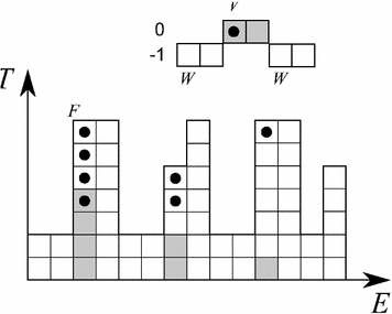
.  is thus the set of all translations where the image lies between both structuring functions and does not touch
  (Fig. 4).
Fig. 4
Illustration of  (Eq. 8). We consider a function
  from
from  into
into  and the two structuring functions
  and
and  (the origin is on the left pixel of
  ). The result of
  is the set of points of
  marked by a black circle inside
  . We also give the result of the application of the integral valuation (Eq. 13) of
  in gray, i.e. the result of
  (Eq. 15)
 (Eq. 8). We consider a function
  from
from  into
into  and the two structuring functions
  and
and  (the origin is on the left pixel of
  ). The result of
  is the set of points of
  marked by a black circle inside
  . We also give the result of the application of the integral valuation (Eq. 13) of
  in gray, i.e. the result of
  (Eq. 15)
Fig. 5
Example of application of the  (Eq. 10) to detect an exponential profile with Gaussian noise [27]. The first image represents a 1D noisy signal. The second image represents the uncertainty area defined by the 2 SFs
  (lower function) and
  (upper function). The third image shows how well the pattern can fit the signal
 (Eq. 10) to detect an exponential profile with Gaussian noise [27]. The first image represents a 1D noisy signal. The second image represents the uncertainty area defined by the 2 SFs
  (lower function) and
  (upper function). The third image shows how well the pattern can fit the signal
Finally, a third fitting involved in Perret’s HMT is given by:
![$$\begin{aligned} P_{V,W}(F) = \left\{ \left( p,\textstyle {\frac{ |\left\{ q \in S \, | \, V(q)+t\le F(p+q)\le W(q)+t\right\} | }{|S|}}\right) \in E \times \left[ 0,1\right] ~\big |~ t\in T\right\} \end{aligned}$$](/wp-content/uploads/2016/03/A308467_1_En_8_Chapter_Equ10.gif)
where  and
and  is the cardinal of the set
  . Hence,
  does not look for locations where both structuring functions completely fit the image. Instead, it measures at each location how well both structuring functions fit the image by counting, among the points of the image that lies in the support of one of the SF, the ratio of points that fits between both SF (Fig. 5).
![$$\begin{aligned} P_{V,W}(F) = \left\{ \left( p,\textstyle {\frac{ |\left\{ q \in S \, | \, V(q)+t\le F(p+q)\le W(q)+t\right\} | }{|S|}}\right) \in E \times \left[ 0,1\right] ~\big |~ t\in T\right\} \end{aligned}$$](/wp-content/uploads/2016/03/A308467_1_En_8_Chapter_Equ10.gif)
(10)
 and
and  is the cardinal of the set
  . Hence,
  does not look for locations where both structuring functions completely fit the image. Instead, it measures at each location how well both structuring functions fit the image by counting, among the points of the image that lies in the support of one of the SF, the ratio of points that fits between both SF (Fig. 5).
3.2.2 Valuation
Likewise, there are several types of valuations. Formally, a valuation  is a mapping that associates a (grayscale) image (
 ) to any result of a fitting
  . Let
. Let  , the simplest valuation
  , the binary valuation, consists in taking the set of points
  for which there is at least one
  such that
  belongs to
  .
.

Another valuation is the supremal valuation  , which for every point
  of fit couples
  , takes the supremum of
  (Fig. 3):

Finally there is the integral valuation  which instead for every point
  of fit couples
  , uses the length of the interval of
  for which the couples
  fit (Fig. 4).

where  is an appropriate measure of intervals in
  (simply the Lebesgue measure if
  is an interval of
  or
or  ).
).
 is a mapping that associates a (grayscale) image (
 ) to any result of a fitting
  . Let
. Let  , the simplest valuation
  , the binary valuation, consists in taking the set of points
  for which there is at least one
  such that
  belongs to
  .
.
(11)
 , which for every point
  of fit couples
  , takes the supremum of
  (Fig. 3):
(12)
 which instead for every point
  of fit couples
  , uses the length of the interval of
  for which the couples
  fit (Fig. 4).
(13)
 is an appropriate measure of intervals in
  (simply the Lebesgue measure if
  is an interval of
  or
or  ).
).3.3 HMT Definitions
The different combinations of fittings and valuations allow to recover the different definitions of HMT. Let  with
with  and
and  , among others, we mention:


 with
with  and
and  , among others, we mention:
(14)

(15)

(16)

Fig. 6
Grayscale HMT : a original image ( pixels); b couple of structuring functions used within the HMT; c result with Ronse’s, d and Soille’s definition (results are displayed in inverse gray levels and for the sake of clarity,
  value was replaced with
  ) [39]
 pixels); b couple of structuring functions used within the HMT; c result with Ronse’s, d and Soille’s definition (results are displayed in inverse gray levels and for the sake of clarity,
  value was replaced with
  ) [39]
4 Template Matching in Color and Multivariate Images
The extension of the HMT to color and more generally to multivariate images such as multi- and hyper-spectral data, can amplify the application potential of the operator at a significant level. Of particular importance in this context are applications regarding color object detection from color data, target detection from remote sensing data, as well as the detection of challenging celestial objects from astronomical imaging sources.
However, given the multitude of existing approaches for the definition of the grayscale HMT, it is no surprise that the situation is no less clearer with multivariate images. In fact, conversely to grayscale morphological image processing, there is not even a generally accepted color mathematical morphology framework, let alone a standardized multivariate HMT. Nevertheless, the increasingly widespread availability of multivariate images, especially in the context of remote sensing, as well as recent advances in color morphology, have provided the missing impetus that has led to the intensification of the research work on extending the HMT to color, multi- and hyper-spectral data.
We will start this section by first recalling the basic theoretical implications of using multivariate images to the mathematical morphology theory, and elaborate on the difficulties of its extension to this type of images. Then, we will present the different methods that have been developed especially in the past few years for applying the HMT to multivariate images.
4.1 Multivariate Mathematical Morphology
According to the lattice based approach to mathematical morphology [30], digital images are represented as mappings  between the discrete coordinate grid
  and the set of pixel values
  , with
  being a complete lattice. More precisely, imposing a complete lattice structure on an arbitrary set of pixel values
  is possible, if
  is equipped with at least a partial ordering relation which enables the computation of the infimum and supremum of any non-empty subset of
  . Consequently, the morphological operators can be in fact applied to any type of image data, as long as the set of pixel values
  possesses a complete lattice structure. For a detailed account of multivariate morphology the reader is referred to Refs. [14, 33].
 between the discrete coordinate grid
  and the set of pixel values
  , with
  being a complete lattice. More precisely, imposing a complete lattice structure on an arbitrary set of pixel values
  is possible, if
  is equipped with at least a partial ordering relation which enables the computation of the infimum and supremum of any non-empty subset of
  . Consequently, the morphological operators can be in fact applied to any type of image data, as long as the set of pixel values
  possesses a complete lattice structure. For a detailed account of multivariate morphology the reader is referred to Refs. [14, 33].
For instance, in the case of continuous multidimensional grayscale images where  , it suffices to employ the usual comparison operator
  , in order to induce a complete lattice structure on
  . Likewise, the inclusion operator
  can be used with binary images
  . However, if we now consider multivariate images
  for the specific case of color images, it becomes problematic to find an ordering relation for the vectors of
  , due to the fact that there is no universal method for ordering multivariate data. As a result, in the last 15 years several ordering approaches have been explored with the end of extending mathematical morphology to multivariate images, for a detailed survey of which the reader is referred to Ref. [2].
 , it suffices to employ the usual comparison operator
  , in order to induce a complete lattice structure on
  . Likewise, the inclusion operator
  can be used with binary images
  . However, if we now consider multivariate images
  for the specific case of color images, it becomes problematic to find an ordering relation for the vectors of
  , due to the fact that there is no universal method for ordering multivariate data. As a result, in the last 15 years several ordering approaches have been explored with the end of extending mathematical morphology to multivariate images, for a detailed survey of which the reader is referred to Ref. [2].
We briefly recall the main properties of an ordering, i.e.a binary relation  on a set
  being reflexive (
 ), anti-symmetric (
 and
and  ), and transitive (
 and
and  ). An ordering is total if the totality statement (
 or
or  ) holds, partial otherwise. It is a pre-ordering if the anti-symmetry statement does not hold.
 on a set
  being reflexive (
 ), anti-symmetric (
 and
and  ), and transitive (
 and
and  ). An ordering is total if the totality statement (
 or
or  ) holds, partial otherwise. It is a pre-ordering if the anti-symmetry statement does not hold.
Hence, the HMT being a morphological tool, its extension to multivariate images also requires the implication of a vector ordering. We will now proceed to examine various solutions developed for applying the HMT to color or to multivariate data in general.
4.2 HMT Based on a Vector Ordering
Aptoula et al. [6] provide the first study on the theoretical requirements of a vector HMT (VHMT). In detail, the initial step for extending the HMT to multivariate data, consists in defining the erosion and dilation operators for multivariate images in combination with multivariate structuring functions (SF). More precisely, these operators are based on horizontal translations (by a point  ) as well as on vertical ones (by a finite pixel value
  ) as in the grayscale case, the difference is however that pixel values are now multi-dimensional; in particular, given a multivariate image
  :
:

Furthermore, according to the fundamental Refs. [16, 17] of Heijmans and Ronse, translations need to be complete lattice automorphisms ( bijections
  that preserve order, and whose inverse also preserve order). Consequently, the vector ordering
  from which the complete lattice is derived, must be translation invariant. In other words:

Thus one can give the definition of the erosion and dilation respectively of a multivariate image F by a multivariate SF B:


 ) as well as on vertical ones (by a finite pixel value
  ) as in the grayscale case, the difference is however that pixel values are now multi-dimensional; in particular, given a multivariate image
  :
:
(17)
 bijections
  that preserve order, and whose inverse also preserve order). Consequently, the vector ordering
  from which the complete lattice is derived, must be translation invariant. In other words:
(18)

(19)
Stay updated, free articles. Join our Telegram channel

Full access? Get Clinical Tree


