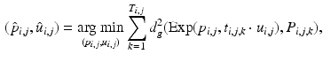
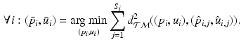
Fig. 1.
A toy example in Euclidean space. Top: (a) Cross-sectional data of two groups, illustrated as red circles and blue squares; (b) the same data with longitudinal information (middle) where points on the same line are observations from one subject; (c) the trajectory space, represented by a slope and an intercept. Every point in this space corresponds to a straight line in (b). Bottom: (d) Trajectories generated by points along the 1st principal component (PC) of standard PCA in trajectory space with  standard deviations (SD); (e) trajectories generated along the 2nd PC (best-viewed in color) (Colour figure online).
standard deviations (SD); (e) trajectories generated along the 2nd PC (best-viewed in color) (Colour figure online).2 Distribution of Trajectories in Euclidean Space
We first illustrate the concept of analyzing populations of trajectories in Euclidean space, which is a trivial case of a Riemannian manifold.
Consider the case of two groups of subjects such that each subject is measured at multiple points in time. Such a data configuration is also referred to as a staggered longitudinal design, see Fig. 1(b). If we ignore the within-subject correlations and model the data with a cross-sectional design, illustrated in Fig. 1(a), the two groups cannot be separated using statistical tests that rely on a comparison of means only (cf. Table 1). Hence, to leverage longitudinal information, we first estimate linear regression models on each subject to summarize its trend. The regression line, a smooth trajectory approximating a subject’s data points, is parameterized the tuple of slope and intercept, which can be represented as a point in the space of trajectories. As shown in Fig. 1(c), representing the data in this trajectory space separates the populations (at least visually) in this example. In fact, Table 1 indicates that including longitudinal information allows us to identify differences between the two groups statistically.
To further analyze the group differences, we explore the distribution of trajectories within the (slope, intercept) space, i.e., the trajectory space. Under a Gaussian assumption, principal component analysis (PCA) is a standard tool to estimate the variance and principal directions of a sample. By applying PCA to (slope, intercept) data, we obtain a representation of the population of trajectories, namely their variances and their principal components. For example, the solid lines with different colors in Fig. 1(c) show the principal components of the two groups, respectively. By moving along these two principal components, we generate new points in the trajectory space such that each point represents a straight line in the original space of the data points. Figure 1(d) and (e) visualize the trajectories along the principal components for different standard deviations. The five trajectories in Fig. 1(d), for instance, show the five points along the first principal component in the trajectory space for each group. This Euclidean case illustrates that the proposed approach is a potentially useful tool in the analysis of longitudinal time-varying data.
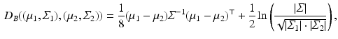
Table 1.
Distances and estimated p-values (10000 random permutations) on toy data using (1) the mean difference in Euclidean space ( ), (2) the Mahalanobis distance (
 ), and (3) the Bhattacharyya distance (
 ) as a test-statistic.
), (2) the Mahalanobis distance (), and (3) the Bhattacharyya distance () as a test-statistic.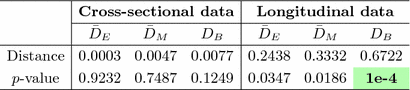 |
Bhattacharyya Distance. Visualization of trajectories along principal directions can qualitatively demonstrate differences between groups. However, to quantitatively assess the differences, we need a suitable distance measure that serves as a test-statistic. An appropriate candidate for this is the Bhattacharyya distance [1], which measures the similarity of two probability distributions. Given two multivariate Gaussians, with means  and covariance matrices
  , the Bhattacharyya distance
  has the closed-form expression
where 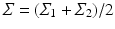 , and
, and  denotes the matrix determinant. The first term in Eq. (1) measures the separability of the distributions w.r.t. their means. It is related to the squared Mahalanobis distance [10], which can be considered a special case of Eq. (1) when the difference between the covariances (as measured by the second term in the summation) is not considered. This additional term makes
  more suitable, compared to the Mahalanobis distance, in cases where the distributions differ in variances. In particular, the Mahalanobis distance is zero when two distributions have equal means. However, as
  only satisfies three conditions of a distance metric (non-negativity, identity of indiscernibles, and symmetry), but lacks the triangle inequality, it is only a semi-metric.
and covariance matrices , the Bhattacharyya distance has the closed-form expression(1)
, and denotes the matrix determinant. The first term in Eq. (1) measures the separability of the distributions w.r.t. their means. It is related to the squared Mahalanobis distance [10], which can be considered a special case of Eq. (1) when the difference between the covariances (as measured by the second term in the summation) is not considered. This additional term makes more suitable, compared to the Mahalanobis distance, in cases where the distributions differ in variances. In particular, the Mahalanobis distance is zero when two distributions have equal means. However, as only satisfies three conditions of a distance metric (non-negativity, identity of indiscernibles, and symmetry), but lacks the triangle inequality, it is only a semi-metric.In fact, Eq. (1) allows us to compute a distance between the two distributions (assuming Gaussianity) in Fig. 1(c), and thereby to define a test-statistic to test for group differences in a permutation testing setup. The null-hypothesis  of the permutation test is that the two distributions (say P, Q) to be tested are the same, i.e.,
  . We estimate the empirical distribution of the test-statistic under
  by repeatedly permuting the group labels of the points in Fig. 1(c), and re-computing
  between the two groups that result from the permuted labels. The p-value under
  then is the proportion of the area under the empirical distribution of samples for which the distance is less than the one estimated for the original (unpermuted) label assignments. In Table 1,
  , tested on the longitudinal data, exhibits the best performance in separating the groups with an estimated p-value of
  1e-4 under 10000 permutations.
of the permutation test is that the two distributions (say P, Q) to be tested are the same, i.e., . We estimate the empirical distribution of the test-statistic under by repeatedly permuting the group labels of the points in Fig. 1(c), and re-computing between the two groups that result from the permuted labels. The p-value under then is the proportion of the area under the empirical distribution of samples for which the distance is less than the one estimated for the original (unpermuted) label assignments. In Table 1, , tested on the longitudinal data, exhibits the best performance in separating the groups with an estimated p-value of 1e-4 under 10000 permutations.3 Distribution of Trajectories on Manifolds
To explore the distribution of trajectories for manifold-valued data, e.g., images or shapes, we need to generalize the statistical test of the previous section from Euclidean space to manifolds. Specifically, let  be a population of longitudinal data on the same manifold, where i is the group identifier, j is the subject identifier, and k identifies the time point. Further assume we have N groups: group i has
  subjects (
 ), and each subject has multiple time points,
 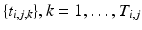 . Our objective is to characterize the distribution of trajectories for each group,
  , i.e., to estimate its variance and principal directions, and to assess whether two groups are significantly different.
be a population of longitudinal data on the same manifold, where i is the group identifier, j is the subject identifier, and k identifies the time point. Further assume we have N groups: group i has subjects (), and each subject has multiple time points, . Our objective is to characterize the distribution of trajectories for each group, , i.e., to estimate its variance and principal directions, and to assess whether two groups are significantly different.Individual Trajectories for Longitudinal Data. To perform statistical tests on subjects with associated longitudinal data, our first step is to summarize the variations within a subject as a smooth trajectory. The parametric geodesic regression approaches for data in Kendall’s shape space [4], or images [7, 13], which generalize linear regression in Euclidean space, provide a compact representation of the continuous trajectory for each subject. The trajectory of subject j from group i is parametrized by the initial point  and the initial velocity
  . This trajectory minimizes the sum-of-squared geodesic distances between the observations and their corresponding points on the trajectory, i.e.,
where  is the geodesic distance and
  denotes the exponential map on some manifold
  [4]. This compact representation,
  , is a point in the tangent bundle
  of
of  .
.  is also a smooth manifold, which can be equipped with a Riemannian metric, such as the Sasaki metric [15]. Since each subject’s longitudinal data is represented as a point on
  , we work in this space, instead of the space of the data points, to perform group testing.
and the initial velocity . This trajectory minimizes the sum-of-squared geodesic distances between the observations and their corresponding points on the trajectory, i.e.,(2)
is the geodesic distance and denotes the exponential map on some manifold [4]. This compact representation, , is a point in the tangent bundle of . is also a smooth manifold, which can be equipped with a Riemannian metric, such as the Sasaki metric [15]. Since each subject’s longitudinal data is represented as a point on , we work in this space, instead of the space of the data points, to perform group testing.Principal Geodesic Analysis (PGA) for Trajectories. We generalize principal geodesic analysis to estimate the variance and the principal directions of trajectories on the tangent bundle for each group. We follow the definitions of the exponential- and the log-map on  in [12] and use the Sasaki metric. Specifically, given two points
  , the log-map outputs the tangent vector such that
  . The exponential map enables us to shoot forward with a given base point and a tangent vector, i.e.,
  . Furthermore, using the log-map, the geodesic distance on
  can be computed as
  .
.
in [12] and use the Sasaki metric. Specifically, given two points , the log-map outputs the tangent vector such that . The exponential map enables us to shoot forward with a given base point and a tangent vector, i.e., . Furthermore, using the log-map, the geodesic distance on can be computed as .Before computing the variance and the principal directions, we first need to estimate the mean of the trajectories for each group. This is done by minimizing the sum-of-squared geodesic distances, for each group, on  as
as
Then, following the PGA algorithm of [5], we compute the variance and principal directions w.r.t. the estimated mean of the trajectories. Specifically, we first compute the tangent vector from the mean of group i to the trajectory of its subject j,  and then calculate the covariance matrix
  . The principal decomposition of
  results in the eigenvalues
  and eigenvectors
  with
with  for group i. As a result, we can identify the distribution of trajectories for each group by
 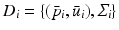 with
with  . By moving along a principal direction, we can generate points on
  , which correspond to trajectories on the manifold of the data points.
as(3)
and then calculate the covariance matrix . The principal decomposition of results in the eigenvalues and eigenvectors with for group i. As a result, we can identify the distribution of trajectories for each group by with . By moving along a principal direction, we can generate points on , which correspond to trajectories on the manifold of the data points.Generalized Bhattacharyya Distance. Since we can characterize the distribution of trajectories on  for each group, to measure the distance between them, we generalize the Bhattacharyya distance from Euclidean space to
  . Again, the distribution
  on
on  , is identified by a mean
  , and a covariance matrix
  with respect to the mean
  .
.
for each group, to measure the distance between them, we generalize the Bhattacharyya distance from Euclidean space to . Again, the distribution on , is identified by a mean , and a covariance matrix with respect to the mean .Related posts:
 Stable Overlapping Replicator Dynamics for Multimodal Brain Subnetwork Identification
 PET Reconstruction with Sparse Image Representation and Anatomical Priors
Stay updated, free articles. Join our Telegram channel

Full access? Get Clinical Tree


