Giulio GAMBAROTA Laboratoire de biophysique, Université de Rennes, France This chapter is dedicated to the measurements of water diffusion in vivo using magnetic resonance imaging (MRI). Since performing in the early days mostly for clinical application in brain, nowadays diffusion-weighted imaging (DWI) is a well-established technique for clinical MRI examinations of different tissues/organs. It has a major role in many therapeutic domains, including oncology and neurology, for both diagnosis and assessment of treatment efficacy. We will first introduce the basic physics of diffusion; then, the measurements of water diffusion using nuclear magnetic resonance (NMR) will be described. Finally, we will illustrate clinical applications of DWI. Here, we present a brief account of the history and physics of diffusion. A simple way to visualize the phenomenon of diffusion is to put a drop of ink into a Petri dish filled with water. Afterward, we observe that the ink particles will spread in time in all directions around their initial position, which can be chosen for simplicity as the origin of a coordinate system (Figure 4.1). The size of the spot will increase with time, as ink particles will diffuse. In general, the phenomenon of diffusion of particles in solution – in the presence of a concentration gradient – was known to scientists of the 19th century. In 1855, the physiologist Adolf Fick described the diffusion of salt in water by the following equation, named Fick’s second law: where ?, the concentration expressed as the number of particles of solute per unit volume of solution, is a function of time and space, that is, ?(?, ?), and ? is the diffusion coefficient. The dimensional analysis of equation [4.1] shows that the diffusion coefficient has dimensions [?] = ?2?-1, that is, ?????ℎ2 ∙ ????-1. Figure 4.1. A drop of ink into a Petri dish filled with water. Upper panel: the ink particles will diffuse in time in all directions. Lower panel: the concentration of ink particles is plotted as a function of time along the radial direction at three time points For simplicity, we consider the diffusion motion just along the x-axis. Under the condition that at time ? = 0, the ink drop is concentrated at the origin, that is, in mathematical terms the initial condition is a Dirac delta function, the solution of equation [4.1] is the Gaussian function: where ?(?, ?) is the concentration and ? is the diffusion coefficient. In Figure 4.1 (lower panel), the concentration is represented at three different time points. Three observations are of interest: (1) this physical system consists of two chemical species (salt and water or ink and water, for instance); (2) strictly speaking, ? is the so-called mutual diffusion coefficient, as we are in a two-component, solvent–solution system; (3) the molecules of solvent diffuse under a macroscopic concentration gradient. We consider now the spot size, which is a metric characterizing how particles diffuse in the solution. The displacement of ink particles could be taken as a measure of this diffusion process. However, when averaged over all particles, the mean displacement will be zero since particles equally spread in all directions. To overcome this problem, the mean square displacement is considered; thus, by taking the displacement of each particle, calculating the square of this value and then averaging over all particles, we obtain a metric that defines and characterizes the phenomenon of diffusion. We can calculate the mean displacement – this is simple, since it is the integral of an odd-function (?) multiplied by an even function (?). Thus, by symmetry arguments the integral is zero, as expected: The calculation of the mean square displacement is more complicated and here we provide just the solution: From this formula, we see that (1) the mean square displacement grows proportionally with time and (2) for a given time, the higher the diffusion coefficient, the bigger the spot size. In 1905, Albert Einstein developed the theoretical framework of the diffusion phenomenon. For the interested reader, the collection of Einstein’s papers related to diffusion are available and translated into English in Einstein and Fürth (1956). Einstein derived the following equation, for particles in a solution: where ? is the ideal gas constant, ?a is the Avogadro constant, ? is the temperature, ? is the viscosity of solvent and ? is the effective radius of the diffusing particles; it should be noted that the Boltzmann constant ? is equal to ?/?a. From equation [4.5], we learn that (1) the diffusion coefficient depends on the temperature: the higher the temperature, the higher the diffusion coefficient; (2) the bigger the particle, the lower the diffusion coefficient; and (3) in contrast to Fick’s law, which requires a concentration gradient for the diffusion to take place, equation [4.5] indicates that particles would undergo a diffusion motion even in the absence of a concentration gradient (!), as long as the temperature is different to 0 K. Thus, the thermal energy of the system drives a constant, random motion of particles in solution. In the same year, equation [4.5] was independently obtained by the physicist William Sutherland (1905). As part of Einstein’s theory, which was based on the viscosity studies by the physicist George Stokes (1819–1903), equation [4.5] is called the Stokes–Einstein–Sutherland equation. Now let us go back to the ink-water experiment and repeat the same experiment, but instead of using a drop of ink we use a drop of water. What happens to the water molecules contained in the water drop? If we could label these water molecules, we would observe a phenomenon similar to that observed with the ink, that is, the water molecules of the drop would diffuse and mix with the other water molecules in the Petri dish, driven by the thermal energy. All of this occurs in the absence of a concentration gradient as there is one chemical species only, that is, a one-component system. Here, strictly speaking, ? is the so-called self-diffusion coefficient, since the molecules diffuse in an environment of identical molecules. Now, what would be the formula that governs the diffusion behavior of water molecules in water? Einstein found that the mean square displacement was given by the formula: This formula is referred to as the Einstein diffusion equation, and it is valid in the case of diffusion along one dimension. For the case of two-dimensional and three-dimensional diffusion, the formula of the mean square displacement is 〈?2〉 = 4?? and 〈?2〉 = 6??, respectively. The combination of the Einstein diffusion equation [4.6] with the Stokes–Einstein–Sutherland equation [4.5] would provide a new way, as Einstein suggested, to determine the Avogadro constant (by eliminating ? from the two equations and measuring all of the remaining physical variables: the viscosity, the temperature and so on). This is exactly what Perrin (1910) did a few years later and his successful experiments were rewarded with the Nobel Prize in Physics in 1926. One year after Einstein’s work, the physicist Marian Smoluchowski (1906) derived the Einstein diffusion equation using a completely different approach: the concept of random walk, which is nowadays often employed to describe self-diffusion processes. Figure 4.2. Example of 2D random walk of four particles. Left panel: four particles start at the origin of the coordinate system and undergo 50 steps in random directions. Each path is shown in a different color. Right panel: the final position of each particle after 50 steps is illustrated by the gray markers In Figure 4.2, the random walk of four particles is illustrated. In this simple case, the mean square displacement can be determined by taking the average over the four particles of their square displacement (square displacement = the distance squared from the origin). In a real scenario for water molecules: each step corresponds to a collision with neighboring molecules and the number of collisions for a single molecule of water in a second is about 1014 (Feynman 1964). It should be also noted that, keeping in mind that 〈?2〉 is proportional to ??, the displacement of a particle in random motion increases with the square-root of the time Before going to the next section, we take a step back to 1827, when the botanist Robert Brown (1828) observed under the microscope grains of pollen suspended in water that were constantly moving in a random fashion. Where was the energy animating these microscopic particles coming from? Were these particles a living organism? Intrigued by his first observations, Brown conducted a series of experiment to further investigate this phenomenon. He concluded that no biological factor was associated to this constant, random motion, since he observed that microscopic particles obtained from stones and suspended in a fluid would display a similar motion. Simply put, Brown took the life out of this random motion, which was later called “the Brownian motion”. Almost a century later, Einstein demonstrated that the random motion of these particles (whether grains of pollen or stone powder) was due to the collision with water molecules and the thermal energy of the system was responsible for this random motion. At last, the scientific saga of Brownian motion that started in 1828 found its end with Einstein’s work in 1905. Further details, information and anecdotes illustrating the impact of Brown’s observations on the scientific community (over a century worth!) can be found in enlightened review articles (Brush 1968; Maiocchi 1990; Haw 2002; Duplantier 2006; Bigg 2008). Already in the very early NMR studies, such as the Spin echoes article by Erwin Hahn in 1950, the effect of the diffusion on the MR signal was detected and investigated (Hahn 1950). Simply put, the random motion of water molecules, in the presence of magnetic field inhomogeneity, resulted in a loss of signal. Hahn indeed observed that the diffusion of water molecules generated a signal attenuation, which could be written as: where ?0 is the signal in the absence of the magnetic field gradient ?, ?? is the echo time, ? is the diffusion coefficient and γ is the gyromagnetic ratio. It is important to notice that in the experimental apparatus employed by Hahn, the magnetic field gradient ? originated from the intrinsic inhomogeneity of the static magnetic field ?0. In 1954, Carr and Purcell (1954) conducted more detailed investigations with the dual aim of (1) reducing the confounding factor introduced by the diffusion in the measurement of ?2 relaxation time and (2) measuring the diffusion coefficient of water. For the first aim, they introduced the idea of using a train of 180° pulses. For achieving the second aim, they applied a magnetic field gradient of 0.28 gauss/cm, generated with two circular turns of current-carrying wire. The gradient was always on throughout the measurement. The measured value of the diffusion coefficient of water at 25°C was equal to 2.5 × 10⁻⁵ cm2⁄s. They concluded that: all methods for measurement of diffusion depend on somehow “labeling” molecules. To the extent that the ‘label’ has a negligible effect on the diffusion process itself, a method may be said to measure truly the “self-diffusion” constant. In the method here described a molecule is in effect labelled by the direction of the nuclear magnetic moment it carries; a more innocuous label would be difficult to imagine. The major methodological improvement in the measurement of diffusion coefficients was proposed by Stejskal and Tanner in 1965. This approach, designed to eliminate certain experimental limitations of the method used by Carr and Purcell, represents the basis of diffusion MRI measurements nowadays. Stejskal and Tanner proposed the use of magnetic field gradient pulses, in contrast to the previous method where the magnetic field gradient was continuously on throughout the measurement. The gradient pulses are illustrated in Figure 4.3. Figure 4.3. The magnetic field gradient pulses employed in the Stejskal and Tanner method. Upper panel: G is the strength of the gradient pulse and δ the duration. Five time intervals are identified. Lower panel: the total magnetic field (?) as a function of the position along the x-axis. Two stationary water molecules, depicted on the x-axis, are located in position ?1 and ?2. In the absence of gradient pulses (time interval 1, 3 and 5), the total magnetic field is equal to the applied static magnetic field ?0 We will analyze in detail the effect of gradient pulses, taken for simplicity along the x-direction, on the spin precession and therefore on the NMR signal. It should be pointed out that the direction of the magnetic field generated by a gradient pulse is always along the z-direction. For a ?x (?y or ?z) gradient, it is just the magnetic field strength that changes linearly along the x-direction (y-direction or z-direction). We consider five time intervals, as indicated in Figure 4.3. One water molecule is located in ?1 and another in ?2, along the x-axis. For the sake of clarity, we focus on one hydrogen nucleus only on each water molecule. We denote with ?1 (?2) the spin of one hydrogen nucleus belonging to the water molecule located in ?1 (?2). In the first time interval, in the absence of a gradient, the magnetic field along the x-axis will be uniform and equal to the static applied magnetic field ?0 (Figure 4.3, lower panel). During the second interval, a gradient pulse of strength ? and duration ? is applied; the total magnetic field ? varies linearly along the x-axis. Thus, the two water molecules will experience a different magnetic field and their spins will precess at different angular frequency, as dictated by the Larmor equation, ? = ??, where ? is the angular frequency, ? the gyromagnetic ratio and ? the total magnetic field. The spin ?2 will precess faster than the spin ?1, since it experiences a stronger magnetic field. As a result of their different resonance frequency, at the end of the second interval there will be a dephasing between ?1 and ?2, which can be calculated as follows. The relation between the phase ? and angular frequency is ? = ?/?, where ? is the time. Thus, ? = ?? = ???. Neglecting the contribution of ?0, since this contribution is similar for ?1 and ?2, the magnetic field in ?1 is ??1 and in ?2 is ??2. At the end of the gradient pulse (? = ?), the phase acquired by the spin ?1 is ?1 = ???1? and for the spin ?2 is ?2 = ???2?. In the third interval, the dephasing is not changing, as ?1 and ?2 precess at the same angular frequency. During the fourth interval, the spin ?1 will precess faster than the spin ?2. At the end of the second gradient pulse, this gradient has induced a phase equal to ?1 = −???1? for ?1 and ?2 = −???2? for ?2; in other words, a phase equal and opposite to the one induced by the first gradient. Thus, for stationary spins, this second gradient has compensated the dephasing induced by the first gradient. During the fifth interval, as ?1 and ?2 are precessing at the same angular frequency and, more importantly, have the same phase. This is the case for stationary, nondiffusing water molecules. What happens in the presence of diffusion? The water molecules will change position (during the third interval, for example, and the new position is For a general formulation of the problem in three dimensions, we consider a magnetic field gradient ? applied along an arbitrary direction. The resonance angular frequency is given by: where ? is the position of the molecule. Given that in general ? = ??/??, by integrating this equation we obtain the general formula of the gradient-induced phase for any type of gradient shape (trapezoidal or sinusoidal shape, for example) and timings: In the case of a rectangular gradient along the x-axis, the integral can be easily solved and we find back the formulae of ? previously developed for ?1 and ?2. We are now ready to set up an experiment for measuring the diffusion coefficient of water using NMR. Following Stejskal and Tanner, we include two gradient pulses into a spin-echo sequence to obtain the pulsed gradient spin echo (PGSE) scheme, as shown in Figure 4.4. It should be noted here that the polarity of the second gradient is the same as that of the first gradient – in contrast to the scheme of Figure 4.3 – since the refocusing RF pulse has the effect of reversing the phase induced by the first gradient. Figure 4.4. The pulsed gradient spin echo (PGSE) sequence proposed by Stejskal and Tanner in 1965. TE is the echo time; G and δ are the strength and duration of the diffusion sensitizing gradient, respectively. Increasing the diffusion time Δ comes at the expense of an increased TE The PGSE scheme is the most commonly used approach nowadays. Other ways to generate a diffusion-weighted (DW) signal include: (1) the stimulated echo (PGSTE) scheme (Tanner 1970), shown in Figure 4.5, where the gradients are positioned during the TE/2 time intervals; (2) the double echo; and (3) the steady-state free precession (SSFP) (Buxton 1993). When comparing the PGSTE to PGSE: the disadvantage of the PGSTE is the well-known 50% signal loss compared to the PGSE (Tanner 1970). On the other hand, the advantage of the PGSTE is that the time interval Δ, also called diffusion (or observation) time, can be extended without increasing the echo time. In other words, longer diffusion times will not yield a signal loss from ?2 relaxation decay when using the PGSTE. We will see later that varying the diffusion time could be useful for investigations of tissue microstructure. It should be noted that magnetic field gradient pulses are ubiquitous in the MRI sequences, in particular for the spatial encoding of the MR signal. When gradient pulses are employed to generate dephasing of diffusing spins, they are typically called “diffusion-sensitizing gradients”. Figure 4.5. The pulsed gradient stimulated echo (PGSTE) sequence proposed by Tanner in 1970. The stimulated pulse sequence consists of three 90° pulses and yields 50% of the signal compared to spin-echo sequence. The TM is the so-called mixing time. Here, the diffusion time Δ can be increased without increasing the TE In general, the signal intensity for an MR diffusion experiment can be written as:
4
The Basics of Diffusion and Intravoxel Incoherent Motion MRI
4.1. Introduction
4.2. The history and physics of diffusion


 . This is in contrast to the displacement of a particle moving with a constant velocity along a straight line, where the displacement increases with the time ?.
4.3. Diffusion and NMR
4.3.1. First NMR measurements of diffusion

4.3.2. Measurements of diffusion with pulsed gradients: the Stejskal and Tanner method

 and
and  ); the dephasing induced by the second gradient ?1 = −??
 ? and ?2 = −??
 ? will not compensate the one induced by the first gradient and we will observe a signal loss.


Related posts:

Stay updated, free articles. Join our Telegram channel

Full access? Get Clinical Tree


