Fig. 1.1
Optical coherence tomography (OCT) generates cross-sectional or three dimensional images by measuring the magnitude and echo time delay of light. Data is composed of axial scans (A-scans) which are measurements of backreflection or backscattering versus delay. Cross-sectional images (B-scan) are generated by transverse scanning the OCT beam, acquiring a series of axial scans. Three dimensional volumetric data sets (3D-OCT) are generated by raster scanning, acquiring a series of cross-sectional images (B-scans)
OCT is a powerful imaging technology in medicine because it performs an “optical biopsy”; it provides a real time, in situ visualization of tissue microstructure and pathology, without the need to remove and process specimens [2, 3]. Although histopathology is the gold standard for the assessment of pathology, it requires tissue excision, fixation, embedding, microtoming and staining. OCT has applications in several general clinical situations:
1.
Where conventional excisional biopsy is hazardous or impossible. Applications include imaging the retina in ophthalmology or coronary arteries in cardiology.
2.
Where excisional biopsy has sampling error. Histopathology of biopsy specimens is the gold standard for diagnosis of many diseases including cancer, however, if excisional biopsy misses the lesion, then there is a false negative. OCT can guide excisional biopsy to reduce the number of biopsies required and to improve sensitivity by reducing sampling errors. If sufficient sensitivity and specificity can be achieved, OCT may be used to diagnose pathology in real time. Since imaging is performed in situ, OCT has the advantage that much larger regions of tissue can be assessed than with excisional biopsy.
3.
For the guidance of interventional procedures. The ability to see cross sectional and three dimensional structure enables the guidance of procedures such as stent placement in intravascular imaging. In ophthalmology, OCT can visualize changes in retinal structure and markers of disease, such as neovascularization or edema, to assess progression or pharmaceutical treatment response. The ability to see beneath the tissue surface enables guidance of ablative therapies such as laser or radio frequency ablation, as well as surgical and microsurgical procedures.
4.
For performing functional measurement and imaging. Doppler OCT enables quantitative measurement of blood flow. OCT angiography enables visualization of vasculature. Polarization sensitive OCT enables measurement of birefringence, a marker for cellular and subcellular organization.
Although the imaging depth of OCT is limited by attenuation from light scattering, coupled with medical devices such as catheter, endoscopic, laparoscopic, or needle delivery instruments, OCT can be used to access luminal organ systems such as the coronary arteries, GI tract and airways, as well as solid organs and masses.
OCT has become a standard of care in clinical ophthalmology and promises to have a powerful impact on intravascular imaging as well as other many other clinical specialties and research applications ranging from diagnosis of neoplasia to enabling new minimally invasive therapies or surgical procedures. This chapter reviews the history and early development of OCT including the translation process of ex vivo imaging studies, preclinical imaging in animals and the first studies in patients. We present a simplified review of key technological developments that have enabled the use of OCT in intravascular imaging and other applications beyond ophthalmology. Finally, we present an overview of commercial activities in the development of intravascular OCT. Commercialization is a key step in making advances available to the wider clinical community, where new methodologies can ultimately impact clinical care. A more rigorous description of the Physics of Cardiovascular OCT is presented in Chap. 2 and a discussion of Future Developments in OCT is presented in Chap. 15.
1.2 OCT and Ultrasound
OCT has features which are common to both ultrasound and microscopy. Therefore, it is helpful to begin by comparing OCT to these modalities. Figure 1.2 shows the resolution and imaging depth for OCT, ultrasound and microscopy. The resolution of clinical ultrasound imaging is typically 0.1–1 mm and depends on the frequency of the sound wave (3–40 MHz) used for imaging [4–6]. Sound waves at ultrasound frequencies below 10 MHz are transmitted with minimal absorption in biological tissue and it is possible to image structures deep in the body. High frequency ultrasound has been used for intravascular imaging as well as research applications. Resolutions of 15–20 μm and finer have been achieved with frequencies above 100 MHz. However, these high frequencies are strongly attenuated in biological tissues and imaging depths are limited to only a few millimeters.
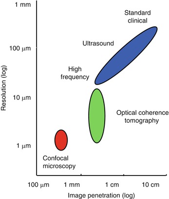
Fig. 1.2
Image resolution and depth. Clinical ultrasound achieves deep imaging depths, but with limited resolution. Higher sound frequencies improve resolution, but increased ultrasonic attenuation reduces imaging depth. Confocal microscopy has submicron resolution, but because it is difficult to reject unwanted scattered light, the imaging depth is a few hundred microns in most tissues. OCT axial image resolution ranges from 1 to 20 μm, according to the coherence length of the light source. In most biological tissues, OCT imaging depth is limited to ~2 mm by attenuation from optical scattering
Microscopy and confocal microscopy are examples of imaging techniques which have extremely high transverse image resolutions of 1 μm or finer. Imaging is typically performed in an en face plane and resolutions are determined by optical diffraction. The imaging depth in biological tissue is limited because image signal and contrast are significantly degraded by unwanted scattered light. In most biological tissues, imaging can be performed to depths of only a few hundred microns.2
OCT fills the gap between ultrasound and microscopy. The axial image resolution in OCT is determined by the bandwidth of the light source. OCT technologies have axial resolutions ranging from 1 to 20 μm, approximately 10 to 100 times finer than standard ultrasound imaging. The high resolution of OCT imaging enables the visualization of tissue morphology. OCT has become a clinical standard in ophthalmology, because the transparency of the eye provides easy optical access to the retina, non-contact high-resolution imaging is possible and there is a dearth of other alternative technologies than can acquire quantitative depth information about the retina [7]. The principal limitation of OCT is that light is highly scattered by most tissues and attenuation from scattering limits the imaging depths to ~2 mm in most tissues. However, because OCT uses fiber optics, it can be integrated with a wide range of medical instruments that can bring the light to the tissue region of interest. Instruments such as catheters, endoscopes, laparoscopes, or needles enable imaging in luminal organ systems or even solid tissues inside the body.
OCT imaging is analogous to ultrasound imaging, except that it uses light instead of sound. There are several different detection methods for performing OCT, but essentially imaging is performed by measuring the magnitude and echo time delay of backreflected or backscattered light from internal microstructures in materials or tissues. OCT images are two-dimensional or three-dimensional data sets which represent optical backreflection or backscattering in a cross-sectional plane or 3D volume. Ultrasound and OCT are analogous in that when a beam of sound or light is incident into tissue, it is backreflected or backscattered differently from structures which have varying acoustic or optical properties, as well as from boundaries between structures. The dimensions of these internal structures can be determined by measuring the “echo” time it takes for sound or light to travel different axial distances.
In ultrasound imaging, the axial measurement of distance or depth is called A-mode scanning, while cross-sectional imaging is called B-mode scanning. Volumetric or 3D imaging can be performed by acquiring multiple B-mode images. The principal difference between ultrasound and optical imaging is the extremely high speed of light and the fact that light has a much shorter wavelength than sound. The speed of sound in tissue is ~1,500 m/s, while the speed of light is approximately 3 × 10⁸ m/s. The measurement of distances with a 100 μm resolution, a typical resolution for ultrasound imaging, requires a time resolution of ~100 ns which is well within the limits of electronic detection. Ultrasound technology has advanced significantly in recent years with the availability of high performance, low cost analog to digital converters and digital signal processing technology. Unlike sound, the detection of light echoes requires much higher time resolution. Light travels from the moon to the earth in only ~2 s. The measurement of distances with a 10 μm resolution, a typical resolution for OCT imaging, requires a time resolution of ~30 femtoseconds (3 × 10⁻¹⁵ s). A femtosecond is extremely fast; the ratio of one femtosecond to one second is equal to the ratio of one second to the time since the age of dinosaurs. Direct electronic detection is extremely difficult with this time resolution; therefore, measurement methods such as high speed optical gating, optical correlation or interferometry are used.
1.3 Measuring Optical Echoes
1.3.1 Photographing Light in Flight
The use of optical echoes to visualize internal structure in biological tissue was proposed more than 40 years ago by Michel Duguay in 1971 [8, 9]. These pioneering studies demonstrated an ultrafast optical shutter using the laser induced Kerr effect which could “photograph light in flight”. Figure 1.3 shows a schematic of Duguay’s ultrahigh speed Kerr shutter photographing an ultrashort light pulse propagating though a scattering solution of diluted milk [9]. The Kerr shutter operates by using an intense laser pulse to induce birefringence (the Kerr effect) in an optical medium placed between two crossed polarizers. If the induced birefringence is electronically mediated, it has an extremely rapid response time and the Kerr shutter can achieve picosecond or femtosecond time resolution.
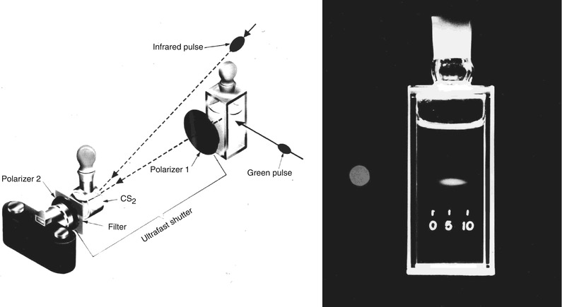
Fig. 1.3
Photographing light in flight. (left) A high speed optical shutter is created using a CS2 cell between crossed polarizers. An intense laser pulse induces transient birefringence (the Kerr effect) to open the shutter. (right) Photograph of an ultrashort laser pulse propagating through a cell of milk and water. The shutter speed was ~10 ps. These early studies suggested that high speed optical gating could be used to see inside biological tissues by rejecting unwanted scattered light (From Duguay [8]; and Duguay and Mattick [9])
Optical scattering limits the ability to image biological tissues, and Duguay proposed that an ultrahigh speed shutter could remove the unwanted scattered light and detect light echoes from inside tissue [9]. Ultrahigh speed optical shutters might be used to “see through” tissues and therefore to non-invasively image internal pathology. The principal limitation of the high speed optical Kerr shutter is that it requires high intensity, short laser pulses to induce the Kerr effect and operate the shutter.
1.3.2 Femtosecond Time Domain Measurement
An alternate method for detecting optical echoes is to use nonlinear optical processes such as harmonic generation, sum frequency generation, or parametric conversion [10–12]. Short light pulses illuminate the tissue and the time delay of backscattered light is detected by nonlinear optical cross correlation, mixing the backreflected light with a time delayed reference pulse in a nonlinear optical material. The nonlinear process can measure the intensity and time delay of the optical signal with a time resolution determined by the pulse duration. Figure 1.4 shows a schematic of how light echoes are detected using nonlinear second harmonic generation cross correlation. The reference pulse is generated by the same laser source and is delayed by a variable time delay ΔT using a mechanical optical delay line. The nonlinear mixing process creates an ultrahigh speed optical gate which is like an optical shutter.
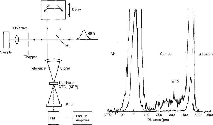
Fig. 1.4
Early demonstration of femtosecond optical ranging in biological systems. (left) Femtosecond echoes of light (signal) are detected using nonlinear second harmonic generation, mixing the signal with a delayed reference pulse. (right) Femtosecond measurement of corneal thickness in a bovine eye ex vivo, showing an axial scan of backscattering versus depth. Using a femtosecond dye laser with a 65 fs pulse duration it was possible to achieve a 15 um axial resolution (in air) with a −70 dB or 10−7 detection sensitivity (From Fujimoto et al. [12])
The ultrahigh speed optical gate enables measurement of the echo magnitude vs time delay of backreflected or backscattered light, the equivalent of an axial scan in an ultrasound. Figure 1.4 shows a measurement of corneal thickness in an in vivo rabbit eye. Very low scattering from the corneal stroma can be detected. The measurement had a 15 μm axial resolution and was performed using 65 femtosecond duration pulses from a femtosecond dye laser at 625 nm wave length. Sensitivities of −70 dB or 10−7 of the incident intensity were achieved. However, these sensitivities were still not high enough to image most biological tissues. Current OCT systems achieve sensitivities 1,000× higher, approaching −100 dB or 10−10 of the incident intensity.
1.3.3 Low Coherence Interferometry
The problem of limited sensitivity can be solved using coherent or interferometric detection. Interferometry is a powerful technique for measuring the magnitude and echo time delay of light with very high sensitivity which has the additional advantage of not requiring short pulse light sources. OCT is based on interferometric imaging and initial embodiments used a classic optical measurement technique known as low coherence interferometry, or white light interferometry, first described by Sir Isaac Newton. Low coherence interferometry was used in photonics to measure optical echoes and backscattering in optical fibers and waveguide devices in the 1980s [13–15]. The first biological application of low coherence interferometry was reported by Fercher et al. in 1988, for the measurement of axial eye length [16]. Different versions of low coherence interferometry were developed for non-invasive measurement in biological tissues [17–20].
Interferometry techniques perform correlation measurements by interfering light that is backscattered from the tissue with light that has traveled a known time delay though a reference path. Interferometry measures the electrical field of the light rather than its intensity. Figure 1.5 shows a schematic diagram of a classic Michelson type interferometer. The incident light is divided into a reference beam and a measurement or signal beam that travels different distances in the two interferometer arms. The path length difference between the interferometer signal and reference arms is ΔL. If the reference path length is scanned, interference fringes will be generated as a function of time. This process can also be understood by noting that scanning the reference arm produces a Doppler shift of the reference field. If a coherent (narrow line width) light source is used, interference will be observed over a long range of path length differences. However, in order to detect optical echoes from a restricted spatial region, a low coherence (broad bandwidth) light source is required. Low coherence light can be characterized as having a temporal (or longitudinal) autocorrelation function whose width is relatively short. The width of the autocorrelation is inversely proportional to the frequency bandwidth of the light. When low coherence light is used, interference is only observed when the measurement and reference path lengths are matched to within the coherence length. The interferometer essentially measures the field autocorrelation of the light. The magnitude and echo time delay of light can be measured by scanning the reference arm and demodulating, or detecting the interference signal. The coherence length of the light source determines the axial image resolution.3 Shorter coherence lengths corresponding to broadband light sources provide finer resolution.
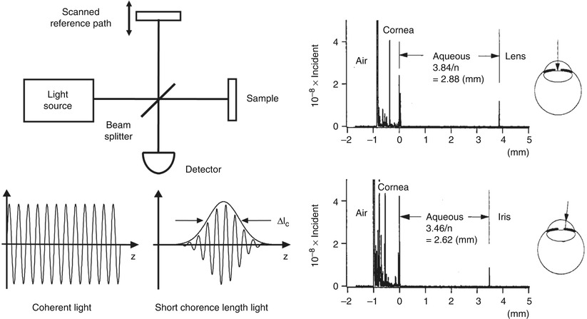
Fig. 1.5
Low coherence interferometry for measuring optical echoes. (left) Backreflected or backscattered light signals are interferred with light from a scanning reference path delay. When low coherence length light is used, interference is only observed with the path lengths are matched to within the coherence length. The interferometer output is detected as the reference path delay is scanned (time domain detection). Axial scan (A-scan) information is obtained by demodulating the inreference signal. (right) Measurement of the anterior chamber in an bovine eye ex vivo. A 10 μm axial resolution was achieved using a low coherence diode light source at ~800 nm. Interferometry enables high sensitivity detection of optical echoes and is the basis for optical coherence tomography (From Huang et al. [21])
Figure 1.5 shows an early ex vivo measurement of the anterior chamber of the bovine eye with a 10 μm axial resolution using an 800 nm wavelength, low coherence diode light source with a 29 nm bandwidth [21]. Sensitivities of −100 dB or 10−10 of the incident intensity were achieved. Scanning the beam in the transverse direction yielded information on different structures, such as the lens and iris. The axial measurements of backscatter versus depth using low coherence interferometry provided the foundation for optical coherence tomography. Low coherence interferometry has the advantage that is can be performed without requiring short pulses of light. Since interferometry measures the electric field rather than the intensity, it is equivalent to heterodyne detection in optical communication. Stated another way, interferometry essentially generates a product of electric fields. Weak signals E Signal (t) are multiplied by a strong reference electrical field E Reference (t) to generate an interference output that is proportional to E Signal (t) × E Reference (t). This multiplication produces homodyne or heterodyne gain and very high, shot noise limited sensitivities (limited by the quantum nature of light) can be achieved and the effects of thermal and other electronic noise sources can be reduced. In addition, since the intensity is proportional to the square of the electric field, very high dynamic ranges are possible because a 10× dynamic range for field corresponds to a 100× dynamic range for intensity. A more comprehensive description of how OCT works can be found in Chap. 2 on the Physics of Cardiovascular OCT.
1.4 The Development of OCT
1.4.1 Early OCT Technology and Systems
Optical coherence tomography imaging was demonstrated in 1991 by Huang et al. [1]. A similar imaging concept was also proposed independently in 1991 by Tanno in Japan [22]. Figures 1.6 and 1.7 show the first OCT images of the retina and human coronary artery ex vivo with corresponding histology [1]. These examples demonstrate OCT imaging in transparent as well as optically scattering tissues. Imaging was performed with 15 μm axial resolution in tissue at 830 nm wavelength. The image is displayed using a log false color scale with a signal level ranging from ~ −60 (red color) to −90 dB (dark blue color) of the incident intensity. The OCT image of the retina in Fig 1.6 shows the contour of the optic nerve head as well as retinal vasculature near the nerve head. The retinal nerve fiber layer can also be visualized emanating from the optic nerve head. This image was ex vivo and postmortem retinal detachment is evident. The OCT image of the coronary artery in Fig. 1.7 shows fibro-calcific plaque on the right of the specimen and fibroatheromatous plaque on the left. The plaque scatters light and therefore attenuates the OCT beam, limiting the image penetration depth below it.
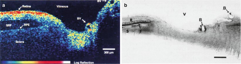
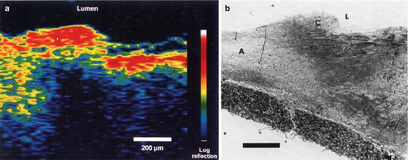
Fig. 1.6
OCT image of the human retina ex vivo (a) and corresponding histology (b). Imaging was performed with 15 μm axial resolution at 830 nm wavelength. The OCT is displayed using a log false color scale ranging from –60 to –90 dB of the incident light intensity. The OCT shows the optic nerve head contour and vasculature. The retinal nerve fiber layer is visualized and there is postmortem retinal detachment, with subretinal fluid accumulation (From Huang et al. [1])
Fig. 1.7
OCT image of human artery ex vivo (a) and corresponding histology (b). The OCT shows fibro-calcific plaque (right three-quarters of specimen) and fibroatheromatous plaque (left side of specimen). The fatty-calcified plaque scatters light, limiting the image penetration depth (From Huang et al. [1])
Optical coherence tomography has the advantage that it can be implemented using fiber optic components and integrated with a wide range of medical devices. OCT systems can be divided into an imaging engine or console (consisting of an interferometer, light source, detector, and support electronics) and imaging devices or probes. Early OCT imaging engines employed time domain detection (TD-OCT) with an interferometer using a low coherence light source and scanning reference delay arm. Figure 1.8 shows an example of a TD-OCT system using a fiber optic Michelson type interferometer with time domain detection. There are many different embodiments of the interferometer and imaging engines which have different power delivery and detection efficiency advantages [23].
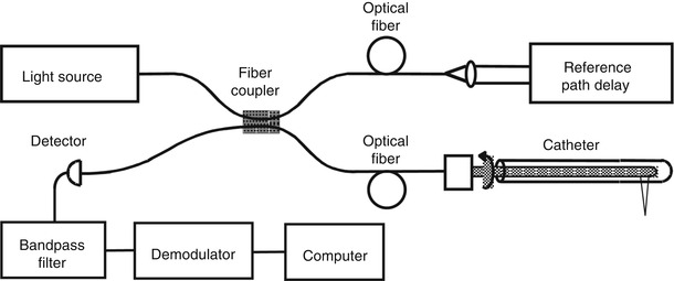
Fig. 1.8
OCT uses photonics and fiber optics technology. This schematic shows a Michelson interferometer implemented using fiber optics. The probe may be interfaced to a variety of medical imaging devices. OCT interferometers can be built in many different configurations depending on design requirements
1.4.2 Ophthalmic OCT Imaging
Because the eye is optically transparent and optical imaging methods were already widely used in ophthalmology, many of the earliest OCT studies were in the eye. The first in vivo retinal images were obtained independently in 1993 by Swanson et al. [24] and Fercher et al. [25]. Figure 1.9 shows an early in vivo OCT image of the normal human retina from Hee et al. in 1995 [26]. Imaging was performed with ~10 μm axial resolution in tissue at ~800 nm wavelength. The nerve fiber layer as well as other architectural features can be visualized with higher resolution than was previously possible. The high detection sensitivity of OCT enables imaging structures such as the retina which are nominally transparent and have very low optical scattering. For retinal imaging, safety standards govern the maximum permissible light exposure and set limits for OCT imaging speeds [24, 26]. Typical retinal images have signal levels −50 to −90 dB below the incident intensity, but are easily visualized using incident power levels that are well within safe exposure limits.
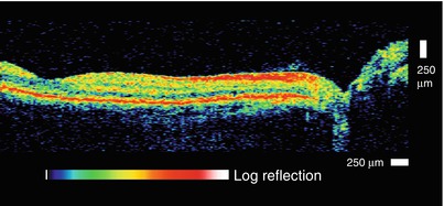
Fig. 1.9
OCT image of the normal human retina in vivo. An early OCT image of the normal human retina in vivo. The OCT has 10 μm axial resolution and was acquired at 800 nm wavelength. The retinal pigment epithelium, choriod, and retinal nerve fiber layers are visible as highly backscattering layers. OCT can noninvasively visualize and quantitatively measure retinal pathology and has become a standard of care in ophthalmology (From Hee et al. [26])
The earliest clinical studies with OCT were performed in ophthalmology, and OCT has had an extremely large clinical impact in this specialty. Early clinical studies investigated OCT for the diagnosis and monitoring of a variety of macular diseases [27], including macular edema [28, 29], macular holes [30], central serous chorioretinopathy [31], and age-related macular degeneration and choroidal neovascularization [32]. The retinal nerve fiber layer thickness, an indicator of glaucoma, can be quantified in normal and glaucomatous eyes and correlated with conventional measurements of the optic nerve structure and function [33, 34]. Many of the measurement protocols that were developed in these early studies were adopted in current OCT ophthalmic instruments [7]. OCT is a powerful technique in ophthalmology because it can identify markers of early disease at treatable time points before visual symptoms and irreversible vision loss occurs. Furthermore, repeated imaging can be performed to track disease progression or monitor the response to therapy.
The important process of translating OCT research into the commercial world began in 1992 when an MIT startup company called Advanced Ophthalmic Devices was founded. Advanced Ophthalmic Devices was acquired by Carl Zeiss Meditec in 1994 and Zeiss introduced its first commercial product for ophthalmic diagnostics in 1996. Early instruments had an axial resolution of 10 μm and an imaging speed of 100 A-scans per second. A third generation ophthalmic instrument, the Stratus OCT, was introduced in 2002 which had similar resolution, but a faster speed of 400 A-scans per second. The increased speed enabled an increase in image pixel density. The large number of published clinical studies from previous generation instruments, coupled with technological improvement helped drive the clinical adoption of OCT. By the mid 2000’s, OCT became the standard of care in ophthalmology and is considered essential for the diagnosis and monitoring of many retinal diseases as well as glaucoma [7]. With increases in imaging speed provided by spectral/Fourier domain detection (see later section of this chapter), many companies entered the ophthalmic marketplace in the mid 2000s. It is estimated that worldwide, approximately 30 million ophthalmic imaging procedures are currently performed annually [35].
1.4.3 Beyond Ophthalmology to Intravascular and Endoscopic Imaging
In OCT applications, detection sensitivity and tissue optical properties are especially important because light is highly attenuated by scattering and absorption, governing the imaging depth. The eye has the advantage that the path from the cornea to the retina (aqueous, lens, and vitreous) is relatively transparent. Although the retina is nominally transparent, it backscatters a small amount of light, which is detected to form OCT images. Early ophthalmic OCT imaging used 800 nm wavelength light because this wavelength minimizes absorption by water in the lens and vitreous. The use of longer wavelengths for OCT imaging was an important step because it reduced scattering and increased image penetration depths [3, 36, 37]. Figure 1.10 shows an early example from Brezinski et al. 1996 showing OCT imaging in a human epiglottis ex vivo, comparing imaging at 800 nm and 1,300 nm wavelengths [3]. At wavelengths shorter than ~1,100 nm, the dominant absorbers in most tissues are melanin and hemoglobin, which absorb at visible and near infrared wavelengths [38]. Water absorption has a peak at 1,450 nm and is extremely high for wavelengths longer than 1,900 nm. In most tissues, scattering at near infrared wavelengths is one to two orders of magnitude higher than absorption (except at the highest absorption peaks), and scattering decreases for longer wavelengths. Therefore, imaging at 1,300 nm improved image penetration and has become a standard wavelength for most OCT applications outside of ophthalmology.
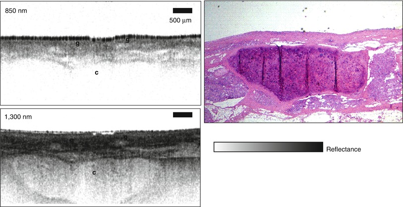
Fig. 1.10
OCT in scattering tissues is possible using long wavelengths which are less attenuated by scattering. OCT of the human epiglottis ex vivo at 850 and 1,300 nm wavelength. Superficial glandular structures (g) are visualized with both 850 and 1,300 nm wavelength, but underlying cartilage (c) is better visualized with longer 1,300 nm wavelength. Scale = 500 μm (From Brezinski et al. [3])
Early studies by Schmitt et al. investigated the mechanisms of OCT image contrast which are related to tissue optical properties [36, 39]. In OCT images, tissue structures are visible because they have different optical scattering properties. OCT images show true tissue dimensions (correcting for index of refraction and beam refraction effects) and do not suffer from processing artifacts as in histology. However if the OCT image is displayed using a false color scale, the colors represent different optical properties and not necessarily different tissue morphologies. Histological sections are stained in order to produce selective contrast between different tissue structures. There are multiple histological stains available which are highly specific. OCT relies on intrinsic differences in optical properties of different tissues to produce image contrast. On one hand, this is a limitation because tissue structures, such as cell nuclei, may not have contrast in traditional OCT imaging. However, histology is a time consuming process that requires tissue excision, processing, embedding, sectioning and staining. OCT imaging can be performed on tissue in situ and in real time, without the need for excision.
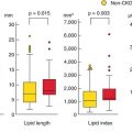
The concept of an “optical biopsy” was explored in several early OCT imaging studies using ex vivo surgical specimens [3, 40–51]. These studies developed the paradigm of comparing OCT imaging to the gold standard of histopathology in order to develop a baseline for the interpretation of OCT images. The concept of using OCT to assess vulnerable plaque was first proposed by Brezinski et al. in 1995 [3, 52]. Figure 1.11 shows an example of one of the first OCT images of plaque ex vivo and corresponding histology from Brezinski et al. 1996 [3]. The OCT image has an axial resolution of ~15 μm in tissue and imaging was performed at 1,300 nm wavelength to optimize imaging depths. The figure shows an unstable plaque characterized by a thin intimal cap layer, adjacent to a heavily calcified plaque with low lipid content. The demonstration that OCT could resolve unstable plaque in ex vivo specimens was an important milestone which helped drive the technological and clinical developments of intravascular OCT imaging.
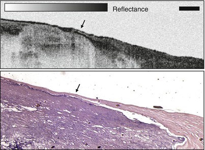
Fig. 1.11
Early OCT image of atherosclerotic plaque ex vivo and corresponding histology. The plaque is highly calcified with relatively low lipid content and a thin intimal cap. This result demonstrated that OCT can resolve morphological features associated with unstable plaques. Scale = 500 μm (From Brezinski et al. [3])
1.4.4 Technology for Catheter and Endoscopic OCT Imaging
The development of flexible fiber optic imaging probes, catheter and endoscopic device technology by Tearney, Bouma et al. at MIT enabled intravascular as well as endoscopic OCT imaging [53, 54]. Figure 1.12 shows one of the first OCT catheter/endoscopes which was a prototype for modern OCT endoscopic probes and intravascular imaging catheters. The catheter/endoscope has a single-mode optical fiber in a hollow rotating torque cable, coupled to a distal lens and microprism that reflects the OCT beam radially outward. The cable and distal optics are contained in a transparent housing. The OCT beam is scanned by rotating the cable to generate a transverse image through luminal structures or hollow organs. Imaging can also be performed in a longitudinal plane by push-pull movement of the fiber optic cable assembly [55]. The early catheter/endoscope shown in Fig. 1.12 had a diameter of 2.9 French or 1 mm, similar to a standard IVUS catheter. The development of catheter imaging devices is challenging because of the simultaneous mechanical, optical and biocompatibility requirements. Early commercial intravascular devices (such as the LightLab Imaging ImageWireTM and HeliosTM occlusion balloon catheters) used micro-optic fabrication methods to create lenses and beam-directing elements which have diameters of optical fibers (80–250 μm), significantly smaller than what can be achieved with IVUS catheters [56].
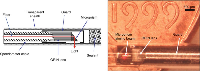
Fig. 1.12
Schematic and photograph of an early OCT catheter/endoscope for intraluminal imaging. A single-mode fiber is housed in a rotating flexible speedometer cable and covered by a transparent plastic sheath. The distal end focuses the beam at ~90° from the catheter axis and scans a rotary pattern and pullback pattern. The catheter diameter is 2.9 French or ~1 mm and is shown on a United States coin for scale. OCT can be integrated with a wide range of diagnostic and interventional devices
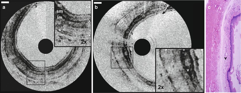
Because of the challenges associated with in vivo intravascular OCT, endoscopic OCT initially progressed more rapidly [54, 57]. Figure 1.13 shows an example of OCT imaging of the rabbit esophagus in vivo and corresponding histology, from Tearney et al. in 1997 [54]. This image demonstrates visualization of esophageal layers including the mucosa (m), submucosa (sm), inner muscularis (im), outer muscularis (om), serosa (s) and used the rotary probe design of Fig. 1.13. The first clinical studies of endoscopic OCT imaging in human subjects were reported by Sergeev et al. in 1997 [57] and Feldchtein et al. in 1998 [58]. These clinical OCT imaging studies were performed with a flexible forward scanning fiber optic probe in the working channel of a standard endoscope, bronchoscope or trocar. The probe was a 1.5–2 mm diameter and used a miniature magnetic optical scanner to image in the forward direction. These early studies demonstrated the feasibility of performing clinical OCT imaging of organ systems such as the esophagus, larynx, stomach, urinary bladder and uterine cervix. However, OCT imaging for neoplasia proved to be challenging because of limitations in image resolution and contrast, with associated difficulty in visualizing nuclei.