Topic
Short description
Sections
Generalities
Introduction;
Derivation of the linear model for color variation;
Derivation of the von Kries model
Result 1
Estimation of the von Kries model
with Application to
Color Correction and
Illuminant invariant image retrieval
Result 2
Dependency of the von Kries model on
the physical cues of the illuminants;
von Kries surfaces;
Application to estimation of
Color temperature and Intensity of an
Illuminant.
Result 3
Dependency of the von Kries model
on the photometric properties of the
acquisition device;
Applications to
Device characterization and to
Illuminant invariant image representation
Conclusions
Final remarks
2 Linear Color Changes
In the RGB color space, the response of a camera to the light reflected from a point  in a scene is coded in a triplet
  =
=  ,
,  ,
,  , where
In Eq. (1),  is the wavelength of the light illuminating the scene,
  its spectral power distribution,
  the reflectance distribution function of the illuminated surface containing
  , and
, and  is the
  -th spectral sensitivity function of the sensor. The integral ranges over the visible spectrum, i.e.
  [380, 780] nm. The values of
  ,
,  ,
,  are the red, green and blue color responses of the camera sensors at point
  .
.
in a scene is coded in a triplet = , , , where(1)
is the wavelength of the light illuminating the scene, its spectral power distribution, the reflectance distribution function of the illuminated surface containing , and is the -th spectral sensitivity function of the sensor. The integral ranges over the visible spectrum, i.e. [380, 780] nm. The values of , , are the red, green and blue color responses of the camera sensors at point .For a wide range of matte surfaces, which appear equally bright from all viewing directions, the reflectance distribution function is well approximated by the Lambertian photometric reflection model [44]. In this case, the surface reflectance can be expressed by a linear combination of three basis functions  with weights
  ,
,  = 0, 1, 2, so that Eq. (1) can be re-written as follows [42]:
where  , the superscript
  indicates the transpose of the previous vector, and
  is the
  matrix with entry
 The response
  captured under an illuminant with spectral power
  is then given by
  . Since the
  ’s do not depend on the illumination, the responses
  and
and  are related by the linear transform
![$$\begin{aligned} \mathbf{p}(x)^T = W [W']^{-1} \mathbf{p'}(x)^T. \end{aligned}$$](/wp-content/uploads/2016/03/A308467_1_En_4_Chapter_Equ3.gif)
Here we assume that  is not singular, so that Eq. (3) makes sense. In the following we indicate the
  -th element of
 ![$$W [W']^{-1}$$](/wp-content/uploads/2016/03/A308467_1_En_4_Chapter_IEq32.gif) by
by  .
.
with weights , = 0, 1, 2, so that Eq. (1) can be re-written as follows [42]:(2)
, the superscript indicates the transpose of the previous vector, and is the matrix with entry captured under an illuminant with spectral power is then given by . Since the ’s do not depend on the illumination, the responses and are related by the linear transform(3)
is not singular, so that Eq. (3) makes sense. In the following we indicate the -th element of by .3 The von Kries Model
The von Kries (or diagonal) model approximates the color change in Eq. (3) by a linear diagonal map, that rescales independently the color channels by real strictly positive factors, named von Kries coefficients.
Despite its simplicity, the von Kries model has been proved to approximate well a color changes due to an illuminant variation [15, 17, 18], especially for narrow-band sensors and for cameras with non-overlapping spectral sensitivities. Moreover, when the device does not satisfy these requirements, its spectral sensitivities can be sharpened by a linear transform [7, 19], so that the von Kries model still holds.
In the following, we derive the von Kries approximation for a narrow-band camera (Sect. 3.1) and for a device with non-overlapping spectral sensitivities (Sect. 3.2). In addition, we discuss a case in which the von Kries model can approximate also a color change due to a device changing (Sect. 3.3).
3.1 Narrow-Band Sensors
The spectral sensitivity functions of a narrow-band camera can be approximated by the Dirac delta, i.e. for each  , where
  is a strictly positive real number and
  is the wavelength at which the sensor maximally responds.
, where is a strictly positive real number and is the wavelength at which the sensor maximally responds.Under this assumption, from Eq. (1), for each  we have
 and thus
This means that the change of illuminant mapping  onto
onto  is a linear diagonal transform that rescales each channel independently. The von Kries coefficients are the rescaling factors
  , i.e. the non null elements
  of
of ![$$W [W']^{-1}$$](/wp-content/uploads/2016/03/A308467_1_En_4_Chapter_IEq42.gif) :
:
we have(4)
onto is a linear diagonal transform that rescales each channel independently. The von Kries coefficients are the rescaling factors , i.e. the non null elements of :(5)
3.2 Non Overlapping Sensitivity Functions
Let  and
and  be two pictures of a same scene imaged under different light conditions. Since the content of
  and
and  is the same, we assume a scene-independent illumination model [52] such that
Now, let us suppose that the device used for the image acquisition has non overlapping sensitivity functions. This means that for each  with
with  ,
,  for any
  . Generally, the spectral sensitivities are real-valued positive functions with a compact support in
  (see Fig. 1 for an example). Therefore non-overlapping sensitivities have non intersecting supports. We prove that under this assumption, the von Kries model still holds, i.e. matrix
 ![$$W[W']^{-1}$$](/wp-content/uploads/2016/03/A308467_1_En_4_Chapter_IEq52.gif) is diagonal.
is diagonal.
and be two pictures of a same scene imaged under different light conditions. Since the content of and is the same, we assume a scene-independent illumination model [52] such that(6)
with , for any . Generally, the spectral sensitivities are real-valued positive functions with a compact support in (see Fig. 1 for an example). Therefore non-overlapping sensitivities have non intersecting supports. We prove that under this assumption, the von Kries model still holds, i.e. matrix is diagonal.Fig. 1
BARNARD2002: spectral sensitivities for the camera Sony DCX-930 used for the image acquisition of the database [8]
From Eq. (6) we have that
i.e. the linear dependency between the responses of a camera under different illuminants is still described by Eq. (3). From Eq. (7) we have that
![$$\begin{aligned}{}[E(\lambda ) F_k(\lambda ) - \sum _{j = 0}^2 \alpha _{kj} E'(\lambda ) F_j(\lambda ) ]^2 = 0. \end{aligned}$$](/wp-content/uploads/2016/03/A308467_1_En_4_Chapter_Equ8.gif)
By minimizing (8) with respect to  and by using the sensitivity non-overlap hypothesis we get the von Kries model. In fact, suppose that
  = 0. The derivative of the Eq. (8) with respect to
  is
is
![$$\begin{aligned} 0 = -E'(\lambda ) F_0(\lambda )[E(\lambda ) F_0(\lambda ) - \sum _{j=0}^{2} \alpha _{0j} E'(\lambda ) F_j(\lambda )]. \end{aligned}$$](/wp-content/uploads/2016/03/A308467_1_En_4_Chapter_Equ47.gif) Thanks to the non-overlapping hypothesis, and by supposing that
Thanks to the non-overlapping hypothesis, and by supposing that  for each
  in the support of
  , we have that
By integrating Eq. (9) with respect to  over
over  , and by solving with respect to
  , we have that
Since  ,
,  and
and  are not identically null,
  is well defined add
  .
.
(7)
(8)
and by using the sensitivity non-overlap hypothesis we get the von Kries model. In fact, suppose that = 0. The derivative of the Eq. (8) with respect to is for each in the support of , we have that(9)
over , and by solving with respect to , we have that(10)
, and are not identically null, is well defined add .Now, we prove that  for any
  . From Eq. (9) we have that
 Putting this expression of
  into Eq. (8) with
  = 0, yields
![$$\begin{aligned} 0 = [\alpha _{01} E'(\lambda ) F_1(\lambda )]^2 + [\alpha _{02} E'(\lambda ) F_2(\lambda )]^2 + 2\alpha _{01}\alpha _{02} E'(\lambda )^2 F_1(\lambda ) F_2(\lambda ) . \end{aligned}$$](/wp-content/uploads/2016/03/A308467_1_En_4_Chapter_Equ49.gif) Since the functions
Since the functions  and
and  do not overlap, the last term at left is null, and
![$$\begin{aligned}{}[\alpha _{01} E'(\lambda ) F_1(\lambda )]^2 + [\alpha _{02} E'(\lambda ) F_2(\lambda )]^2 = 0. \end{aligned}$$](/wp-content/uploads/2016/03/A308467_1_En_4_Chapter_Equ50.gif) By integrating this equation over
By integrating this equation over  we have that
![$$\begin{aligned} \alpha _{01}^2 \int _\Omega [E'(\lambda ) F_1(\lambda )]^2 d\lambda + \alpha _{02}^2 \int _\Omega [E'(\lambda ) F_2(\lambda )]^2 d\lambda = 0, \end{aligned}$$](/wp-content/uploads/2016/03/A308467_1_En_4_Chapter_Equ11.gif)
and since  ,
,  ,
,  ,
,  , are not identically zero, we have that
  . By repeating the same procedure for
  , we obtain the von Kries model.
for any . From Eq. (9) we have that into Eq. (8) with = 0, yields and do not overlap, the last term at left is null, and we have that(11)
, , , , are not identically zero, we have that . By repeating the same procedure for , we obtain the von Kries model.We remark that Eq. (9) has been derived by supposing that  differs from zero for any
  in the compact support of
  . This allows us to remove the multiplicative term
  and leads us to Eq. (9). This hypothesis is reliable, because the spectral power distribution of the most illuminants is not null in the visible spectrum. However, in case of lights with null energy in some wavelengths of the support of
  , Eq. (9) is replaced by
![$$\begin{aligned} E'(\lambda ) E(\lambda )[ F_0(\lambda )]^2 - \alpha _{00} [E'(\lambda )]^2 [F_0(\lambda )]^2 = 0. \end{aligned}$$](/wp-content/uploads/2016/03/A308467_1_En_4_Chapter_Equ51.gif) The derivation of the von Kries model can be then carried out as before.
The derivation of the von Kries model can be then carried out as before.
differs from zero for any in the compact support of . This allows us to remove the multiplicative term and leads us to Eq. (9). This hypothesis is reliable, because the spectral power distribution of the most illuminants is not null in the visible spectrum. However, in case of lights with null energy in some wavelengths of the support of , Eq. (9) is replaced by3.3 Changing Device
A color variation between two images of the same scene can be produced also by changing the acquisition device. Mathematically turns into changing the sensitivity function  in Eq. (1). Here we discuss a case in which the color variation generated by a device change can be described by the von Kries model.
in Eq. (1). Here we discuss a case in which the color variation generated by a device change can be described by the von Kries model.Without loss of generality, we can assume that the sensors are narrow bands. Otherwise, we can apply the sharpening proposed in [18] or [7]. Under this assumption, the sensitivities of the cameras used for acquiring the images under exam are approximated by the Dirac delta, i.e.
where parameter  is a characteristic of the cameras.
(12)
is a characteristic of the cameras.Here we model the change of the camera as a variation of the parameter  , while we suppose that the wavelength
  remains the same. Therefore the sensitivity functions changes from Eq. (12) to the following Equation:
Consequently, the camera responses are
 and thus, therefore the diagonal linear model still holds, but in this case, the von Kries coefficients
  depends not only on the spectral power distribution, but also on the device photometric cues:
, while we suppose that the wavelength remains the same. Therefore the sensitivity functions changes from Eq. (12) to the following Equation:(13)
depends not only on the spectral power distribution, but also on the device photometric cues:(14)
4 Estimating the von Kries Map
The color correction of an image onto another consists into borrow the colors of the first image on the second one. When the color variation is caused by a change of illuminant, and the hypotheses of the von Kries model are satisfied, the color transform between the two pictures is determined by the von Kries map. This equalizes their colors, so that the first picture appears as it would be taken under the illuminant of the second one. Estimating the von Kries coefficients is thus an important task to achieve color correction between images different by illuminants.
The most methods performing color correction between re-illuminated images or regions compute the von Kries coefficients by estimating the illuminants  and
and  under which the images to be corrected have been taken. These illuminants are expressed as RGB vectors, and the von Kries coefficients are determined as the ratios between the components of the varied illuminants. Therefore, estimating the von Kries map turns into estimating the image illuminants. Some examples of these techniques are the low-level statistical based methods as Gray-World and Scale-by-Max [11, 33, 55], the gamut approaches [4, 14, 20, 23, 29, 56], and the Bayesian or statistical methods [26, 41, 47, 50].
and under which the images to be corrected have been taken. These illuminants are expressed as RGB vectors, and the von Kries coefficients are determined as the ratios between the components of the varied illuminants. Therefore, estimating the von Kries map turns into estimating the image illuminants. Some examples of these techniques are the low-level statistical based methods as Gray-World and Scale-by-Max [11, 33, 55], the gamut approaches [4, 14, 20, 23, 29, 56], and the Bayesian or statistical methods [26, 41, 47, 50].The method proposed in [35], we investigate here, differs from these techniques, because it does not require the computation of the illuminants  and
and  , but it estimates the von Kries coefficients by matching the color histograms of the input images or regions, as explained in Sect. 4.1. Histograms provide a good compact representation of the image colors and, after normalization, they guarantee invariance with respect to affine distortions, like changes of size and/or in-plane orientation.
and , but it estimates the von Kries coefficients by matching the color histograms of the input images or regions, as explained in Sect. 4.1. Histograms provide a good compact representation of the image colors and, after normalization, they guarantee invariance with respect to affine distortions, like changes of size and/or in-plane orientation.As matter as fact, the method in [35] is not the only one that computes the von Kries map by matching histograms. The histogram comparison is in fact adopted also by the methods described in [9, 34], but their computational complexities are higher than that of the method in [35]. In particular, the work in [9] considers the logarithms of the RGB responses, so that a change in illumination turns into a shift of these logarithmic responses. In this framework, the von Kries map becomes a translation, whose parameters are derived from the convolution between the distributions of the logarithmic responses, with computation complexity  , where
  is the color quantization of the histograms. The method in [34] derives the von Kries coefficients by a variational technique, that minimizes the Euclidean distance between the piecewise inverse of the cumulative color histograms of the input images or regions. This algorithm is linear with the quantizations
  and
and  of the color histograms and of the piecewise inversions of the cumulative histograms respectively, so that its complexity is
  . Differently from the approach of [34], the algorithm in [35] requires the user just to set up the value of
  and its complexity is
  .
.
, where is the color quantization of the histograms. The method in [34] derives the von Kries coefficients by a variational technique, that minimizes the Euclidean distance between the piecewise inverse of the cumulative color histograms of the input images or regions. This algorithm is linear with the quantizations and of the color histograms and of the piecewise inversions of the cumulative histograms respectively, so that its complexity is . Differently from the approach of [34], the algorithm in [35] requires the user just to set up the value of and its complexity is .The method presented in [35] is described in detail in Sect. 4.1. Experiments on the accuracy and an analysis of the algorithm complexity and dependency on color quantization are addressed in Sects. 4.2 and 4.3 respectively. Finally, Sect. 4.4 illustrates an application of this method to illuminant invariant image retrieval.
4.1 Histogram-Based Estimation of the von Kries Map
As in [35], we assume that the illuminant varies uniformly over the pictures. We describe the color of an image  by the distributions of the values of the three channels red, green, blue. Each distribution is represented by a histogram of
  bins, where
  ranges over {1, …, 256}. Hence, the color feature of an image is represented by a triplet
  of histograms. We refer to
  as color histograms, whereas we name its components channel histograms.
by the distributions of the values of the three channels red, green, blue. Each distribution is represented by a histogram of bins, where ranges over {1, …, 256}. Hence, the color feature of an image is represented by a triplet of histograms. We refer to as color histograms, whereas we name its components channel histograms.Let  and
and  be two color images, with
  being a possibly rescaled, rotated, translated, skewed, and differently illuminated version of
  . Let
. Let  and
and  denote the color histograms of
  and
and  respectively. Let
  and
and  be the
  -th component of
  and
and  respectively. Here fter, to ensure invariance to image rescaling, we assume that each channel
  histogram is normalized so that
  = 1.
= 1.
and be two color images, with being a possibly rescaled, rotated, translated, skewed, and differently illuminated version of . Let and denote the color histograms of and respectively. Let and be the -th component of and respectively. Here fter, to ensure invariance to image rescaling, we assume that each channel histogram is normalized so that = 1.The channel histograms of two images which differ by illumination are stretched to each other by the von Kries model, so that
We note that, as the data are discrete, the value  is cast to an integer ranging over {1, …, 256}.
(15)
is cast to an integer ranging over {1, …, 256}.The estimate of the parameters  ’s consists of two phases. First, for each
  in {1, …, 256} we compute the point
  in {1, …, 256} such that
Second, we compute the coefficient  as the slope of the best line fitting the pairs
  .
.
’s consists of two phases. First, for each in {1, …, 256} we compute the point in {1, …, 256} such that(16)
as the slope of the best line fitting the pairs .The procedure to compute the correspondences  satisfying Eq. (16) is implemented by the Algorithm 1 and more details are presented in [35]. To make the estimate robust to possible noise affecting the image and to color quantization, the contribution of each pair
  is weighted by a positive real number
  , that is defined as function of the difference
  .
.
satisfying Eq. (16) is implemented by the Algorithm 1 and more details are presented in [35]. To make the estimate robust to possible noise affecting the image and to color quantization, the contribution of each pair is weighted by a positive real number , that is defined as function of the difference .The estimate of the best line  could be adversely affected by the pixel saturation, that occurs when the incident light at a pixel causes the maximum response (256) of a color channel. To overcome this problem, and to make our estimate robust as much as possible to saturation noise, the pairs
  with
with  or
or  are discarded from the fitting procedure.
could be adversely affected by the pixel saturation, that occurs when the incident light at a pixel causes the maximum response (256) of a color channel. To overcome this problem, and to make our estimate robust as much as possible to saturation noise, the pairs with or are discarded from the fitting procedure.A least-square method is used to define the best line fitting the pairs  . More precisely, the value of
  is estimated by minimizing with respect to
  the following functional, that is called in [35] divergence:
Here  and
and  indicate the
  -th pair satisfying Eq. (16) and its weight respectively, while
  is the Euclidean distance between the point
  and the line
  .
.
. More precisely, the value of is estimated by minimizing with respect to the following functional, that is called in [35] divergence:(17)
and indicate the -th pair satisfying Eq. (16) and its weight respectively, while is the Euclidean distance between the point and the line .We observe that:
These properties imply that  is a measure of dissimilarity (divergence) between the channel histograms stretched each to other. In particular, if
  is zero, than the two histograms are stretched to each other.
1.
 = 0
= 0 
 , for each
  in {1, …,
  };
};
= 0 , for each in {1, …, };2.
 =
=  .
.
= . is a measure of dissimilarity (divergence) between the channel histograms stretched each to other. In particular, if is zero, than the two histograms are stretched to each other.Finally we notice that, when no changes of size or in-plane orientation occur, the diagonal map between two images  and
and  can be estimated by finding, for each color channel, the best line fitting the pairs of sensory responses
  at the
  -th pixels of
  and
and  respectively, as proposed in [37]. The histogram-based approach in [35] basically applies a least square method in the space of the color histograms. Using histograms makes the estimate of the illuminant change insensitive to image distortions, like rescaling, translating, skewing, and/or rotating.
and can be estimated by finding, for each color channel, the best line fitting the pairs of sensory responses at the -th pixels of and respectively, as proposed in [37]. The histogram-based approach in [35] basically applies a least square method in the space of the color histograms. Using histograms makes the estimate of the illuminant change insensitive to image distortions, like rescaling, translating, skewing, and/or rotating.Figure 2 shows a synthetic example of pictures related by a von Kries map along with the color correction provided by the method described in [35]. The red channel of the image (a) has been rescaled by 0.5, while the other channels are unchanged. The re-illuminated image is shown in (b). Figure 3 shows the red histograms of (a) and (b) and highlights the correspondence between two bins. In particular, we note that the green regions in the two histograms have the same areas. The von Kries map estimated by [35] provides a very satisfactory color correction of image (b) onto image (a), as displayed in Fig. 2c.
Fig. 2
a A picture; b a re-illuminated version of (a); c the color correction of (b) onto (a) provided by the method [35]. Pictures (a) and (c) are highly similar
Fig. 3
Histograms of the responses of the red channels of the pictures shown in Fig. 2a, b: the red channel of the first picture has been synthetically rescaled by 0.5. The two red histograms are thus stretched to each other. The method [35] allows to estimate the stretching parameters, and hence to correct the images as they would be taken under the same light. The green parts highlighted on the histograms have the same area, therefore the bin  in the first histogram is mapped on the bin
  of the second one
in the first histogram is mapped on the bin of the second one4.2 Accuracy on the Estimate
The accuracy on the estimate of the von Kries map possibly relating two images or two image regions has been measured in [35] in terms of color correction. In the following, we report the experiments carried out on four real-world public databases (ALOI [27], Outex [45], BARNARD [8], UEA Dataset [16]). Some examples of pictures from these datasets are shown in Fig. 4 (first and second images in each row).
Each database consists of a set of images (references) taken under a reference illuminant and a set of re-illuminated versions of them (test images). For all the databases, we evaluate the accuracy on the estimation of the the von Kries map  by
by
by(18)
Fig. 4
Examples of color correction output by the approach in [35] for the four databases used in the experiments reported in Sect. 4.2: a ALOI, b Outex; c BARNARD; d UEA. In each row, from left to right: an image, a re-illuminated version of it, and the color correction of the second one onto the first one. The images in (d) have been captured by the same camera
Here  indicates a test image and
  its correspondent reference, while
  is the
  distance computed on the RGB space between
  and the color correction
  of
of  determined by the estimated
  . This distance has been normalized to range over [0,1]. Therefore, the closer to 1
  is, the better our estimate is. To quantify the benefit of our estimate, we compare the accuracy in Eq. (18) with
The value of  measures the similarity of the reference to the test image when no color enhancement is applied.
indicates a test image and its correspondent reference, while is the distance computed on the RGB space between and the color correction of determined by the estimated . This distance has been normalized to range over [0,1]. Therefore, the closer to 1 is, the better our estimate is. To quantify the benefit of our estimate, we compare the accuracy in Eq. (18) with(19)
measures the similarity of the reference to the test image when no color enhancement is applied.The transform  gives the color correction of
  with respect to the reference
  : in fact,
  is the image
  as it would be taken under the same illuminant of
  .
.
gives the color correction of with respect to the reference : in fact, is the image as it would be taken under the same illuminant of .We notice that this performance evaluation does not consider possible geometric image changes, like rescaling, in-plane rotation, or skew. In fact, the similarity between two color corrected images is defined as a pixel-wise distance between the image colors.
In case of a pair of images related by an illuminant change and by geometric distortions, we measure the accuracy of the color correction by the  distance between their color histograms. In particular, we compute the distance
  between the color histograms of
  and
and  before the color correction
and the distance  between the color histograms
  and
and  of
of  and
and  respectively:
Examples of color correction output by the algorithm we described are shown in Fig. 4 for each database used here (third image in each row).
distance between their color histograms. In particular, we compute the distance between the color histograms of and before the color correction(20)
between the color histograms and of and respectively:(21)
4.2.1 ALOI
ALOI [27] (http://staff.science.uva.nl/~aloi/) collects 110,250 images of 1,000 objects acquired under different conditions. For each object, the frontal view has been taken under 12 different light conditions, produced by varying the color temperature of 5 lamps illuminating the scene. The lamp voltage was controlled to be  V with
 {110, 120, 130, 140, 150, 160, 170, 180, 190, 230, 250}. For each pair of illuminants
  with
with  , we consider the images captured with lamp voltage
  as references and those captured with voltage
  as tests.
V with {110, 120, 130, 140, 150, 160, 170, 180, 190, 230, 250}. For each pair of illuminants with , we consider the images captured with lamp voltage as references and those captured with voltage as tests.Figure 5 shows the obtained results: for each pair  , the plot shows the accuracies (a)
  and (b)
  averaged over the test images.
, the plot shows the accuracies (a) and (b) averaged over the test images.We observe that, for  , the accuracy
  is lower than for the other lamp voltages. This is because the voltage
  determines a high increment of the light intensity and therefore a large number of saturated pixels, making the performances worse.
, the accuracy is lower than for the other lamp voltages. This is because the voltage determines a high increment of the light intensity and therefore a large number of saturated pixels, making the performances worse.The mean value of  averaged on all the pairs
  is 0.9913, while that of
  is 0.9961 by the approach in [35]. For each pair of images
  representing a same scene taken under the illuminants with voltages
  and
and  respectively, we compute the parameters
  of the illuminant change
  mapping
  onto
onto  . In principle, these parameters should be equal to those of the map
  relating another pair
  captured under the same pair of illuminants. In practice, since the von Kries model is only an approximation of the illuminant variation, the parameters of
  and
and  generally differ. In Fig. 6 we report the mean values of the von Kries coefficients versus the reference set. The error bar is the standard deviation of the estimates from their mean value.
averaged on all the pairs is 0.9913, while that of is 0.9961 by the approach in [35]. For each pair of images representing a same scene taken under the illuminants with voltages and respectively, we compute the parameters of the illuminant change mapping onto . In principle, these parameters should be equal to those of the map relating another pair captured under the same pair of illuminants. In practice, since the von Kries model is only an approximation of the illuminant variation, the parameters of and generally differ. In Fig. 6 we report the mean values of the von Kries coefficients versus the reference set. The error bar is the standard deviation of the estimates from their mean value.


4.2.2 Outex Dataset
The Outex database [45] (http://www.outex.oulu.fi/) includes different image sets for empirical evaluation of texture classification and segmentation algorithms. In this work we extract the test set named Outex_TC_00014: this consists of three sets of 1360 texture images viewed under the illuminants INCA, TL84 and HORIZON with color temperature 2856, 4100 and 2300 K respectively.
The accuracies  and
and  are stored in Table 2, where three changes of lights have been considered: from INCA to HORIZON, from INCA to TL84, from TL84 to HORIZON. As expected,
  is greater than
  .
.
and are stored in Table 2, where three changes of lights have been considered: from INCA to HORIZON, from INCA to TL84, from TL84 to HORIZON. As expected, is greater than .Fig. 6
ALOI: estimates of the von Kries coefficients
Table 2
Outex: accuracies  and
and  for three different illuminant changes
and for three different illuminant changesIlluminant change |  |  |
|---|---|---|
From INCA to HORIZON | 0.94659 | 0.97221 |
From INCA to TL84 | 0.94494 | 0.98414 |
From TL84 to HORIZON | 0.90718 | 0.97677 |
Mean | 0.93290 | 0.97771 |
4.2.3 BARNARD
The real-world image dataset [8] (http://www.cs.sfu.ca/~colour/), that we refer as BARNARD, is composed by 321 pictures grouped in 30 categories. Each category contains a reference image taken under an incandescent light Sylvania 50MR16Q (reference illuminant) and a number (from 2 to 11) of relighted versions of it (test images) under different lights. The mean values of the accuracies  and
and  are shown in Fig. 7. On average,
  is 0.9447, and
  is 0.9805.
and are shown in Fig. 7. On average, is 0.9447, and is 0.9805.


4.2.4 UEA Dataset
The UEA Dataset [16] (http://www.uea.ac.uk/cmp/research/) comprises 28 design patterns, each captured under 3 illuminants with four different cameras. The illuminants are indicated by Ill A (tungsten filament light, with color temperature 2865 K), Ill D65 (simulated daylight, with color temperature 6500 K), and Ill TL84 (fluorescent tube, with color temperature 4100 K). We notice that the images taken by different cameras differ not only for their colors, but also for size and orientation. In fact, different sensors have different resolution and orientation. In this case, the accuracy on the color correction cannot be measured by the Eqs. (18) and (19), but it is evaluated by the histogram distances defined in Eqs. (20) and (21).
The results are reported in Table 3. For each pair of cameras  and for each illuminant pair
  we compute the von Kries map relating every image acquired by
  under
under  and the correspondent image acquired by
  under
under  , and the accuracies
  and
and  on the color correction of the first image onto the second one. On average, the
  distance between the color histograms before the color correction is 0.0043, while it is 0.0029 after the color correction.
and for each illuminant pair we compute the von Kries map relating every image acquired by under and the correspondent image acquired by under , and the accuracies and on the color correction of the first image onto the second one. On average, the distance between the color histograms before the color correction is 0.0043, while it is 0.0029 after the color correction.Table 3
UEA Dataset: Accuracies  and
and  respectively (a) before and (b) after the color correction.
and respectively (a) before and (b) after the color correction.