Transfer Segmentation

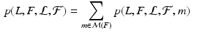
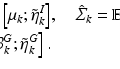
Fig. 1.

Illustration of keypoint transfer segmentation. First, keypoints (white circles) in training and test images are matched (arrow). Second, voting assigns an organ label to the test keypoint (r.Kidney). Third, matches from the training images with r.Kidney as labels are transferred to the test image, creating a probabilistic segmentation. We show the manual segmentation for comparison.

Keypoint matching offers the additional advantage of robustness in establishing correspondences between images with varying field-of-view. This property is important when using manually annotated whole-body scans to segment clinical scans with a limited field-of-view. In clinical practice, the diagnostic focus is commonly on a specific anatomical region. To minimize radiation dose to the patient and scanning time, only the region of interest is scanned. The alignment of scans with a limited field-of-view to full abdominal scans is challenging with intensity-based registration, especially when the initial transformation does not roughly align anatomical structures. The efficient and robust segmentation through keypoint transfer offers a practical tool to handle the growing number of clinical scans.

Figure 1 illustrates the keypoint transfer segmentation. Keypoints are identified at salient image regions invariant to scale. Each keypoint is characterized by its geometry and a descriptor based on a local gradient histogram. After keypoint extraction, we obtain the segmentation in three steps. First, keypoints in the test image are matched to keypoints in the training images based on the geometry and the descriptor. Second, reliable matches vote on the organ label of the keypoint in the test image. In the example, two matches vote for right kidney and one for liver, resulting in a majority vote for right kidney. Third, we transfer the segmentation mask for the entire organ for each match that is consistent with the majority label vote; this potentially transfers the organ map from one training image multiple times if more than one match is identified for this training image. The algorithm also considers the confidence of the match in the keypoint label voting. Keypoint transfer does not require a training stage. Its ability to approximate the organ shape improves as the number of manually labeled images grows.

1.1 Related Work

Several methods have been previously demonstrated for segmenting large field-of-view scans. Entangled decision forests [13] and a combination of discriminative and generative models [8] have been proposed for the segmentation of CT scans. A combination of local and global context for simultaneous segmentation of multiple organs has been explored [11]. Organ detection based on marginal space learning was proposed in [20]. The application of regression forests for efficient anatomy detection and localization was described in [4]. In contrast to previously demonstrated methods, our algorithm does not require extensive training on a set of manually labeled images.

We evaluate our method on the publicly available Visceral dataset [10, 19]. Multi-atlas segmentation on the Visceral data was proposed in [6, 9], which we use as a baseline method in our experiments. Our work builds on the identification of keypoints, defined as a 3D extension [18] of the popular scale invariant feature transform (SIFT) [12]. In addition to image alignment, 3D SIFT features were also applied to study questions related to neuroimaging [17]. In contrast to previous uses of the 3D SIFT descriptor, we use it to transfer information across images.

2 Method

In atlas-based segmentation, the training set includes images 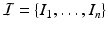$\mathcal {I} = \{I_1, \ldots , I_n\}$ and corresponding segmentations $\mathcal {S} = \{S_1, \ldots , S_n\}$ , where $S_i(x) \in \{1, \ldots , \eta \}$ for $\eta$ labels. The objective is to infer segmentation S for test image I. Instead of aligning training images to the test image with deformable registration, we automatically extract anatomical features from the images and use them to establish sparse correspondences. We identify keypoints that locally maximize a saliency function. In the case of SIFT, it is the difference-of-Gaussians [12]

$\begin{aligned} \{(x_i, \sigma _i)\} = \text {local} \, \mathop {\text {arg max}}\limits _{x,\sigma } | f(x, \kappa \sigma ) - f(x, \sigma ) |, \end{aligned}$

(1)

where

and $\sigma _i$ are the location and scale of keypoint i, $f(\cdot ,\sigma )$ is the convolution of the image I with a Gaussian kernel of variance $\sigma ^2$ , and $\kappa$ is a multiplicative scale sampling rate. The identified local extrema in scale-space correspond to distinctive spherical image regions. We characterize the keypoint by a descriptor

computed in a local neighborhood whose size depends on the scale of the keypoint. We work with a 3D extension of the image gradient orientation histogram [18] with 8 orientation and 8 spatial bins. This description is scale and rotation invariant and further robust to small deformations. Constructing the descriptors from image gradients instead of intensity values facilitates comparisons across subjects.

We combine the 64-dimensional histogram

with the location $F^x \in {\mathbb R}^3$ and scale $F^\sigma \in {\mathbb R}$ to create a compact 68-dimensional representation F for each salient image region. We let

denote the set of keypoints extracted from the test image I and ${\mathcal F}_{\mathcal I}= \{{\mathcal F}_{I_1}, \ldots , {\mathcal F}_{I_n} \}$ denote the set of keypoints extracted from the training images ${\mathcal I}$ . We assign a label to each keypoint in ${\mathcal F}_{I_i}$ according to the organ that contains it, ${\mathcal L}= S_i({\mathcal F}^x)$ for ${\mathcal F}\in {\mathcal F}_{I_i}$ . We only keep keypoints within the segmented organs and discard those in the background. The organ label L is unknown for the keypoints in the test image and is inferred with a voting algorithm as described later in this section.

2.1 Keypoint Matching

The first step in the keypoint-based segmentation is to match each keypoint in the test image with keypoints in the training images. Some of these initial matches might be incorrect. We employ a two-stage matching procedure with additional constraints to improve the reliability of the matches. First, we compute a match ${\mathcal M}(F)_i$ for a test keypoint $F \in F_I$ to keypoints in a training image ${\mathcal F}_{I_i}$ by identifying the nearest neighbor based on the descriptor and scale constraints

$\begin{aligned} {\mathcal M}(F)_i = \mathop {\text {arg min}}\limits _{{\mathcal F}\in {\mathcal F}_{I_i}} \Vert F^D - {\mathcal F}^D \Vert , \ \ \ \text {s.t.} \ \ \varepsilon _\sigma ^{-1} \le \frac{F^\sigma }{{\mathcal F}^\sigma } \le \varepsilon _\sigma , \end{aligned}$

(2)

where we set a loose threshold on the scale allowing for variations up to a factor of $\varepsilon _\sigma = 2$ . We use the distance ratio test to discard keypoint matches that are not reliable [12]. The distance ratio is computed between the descriptors of the closest and second-closest neighbor. We reject all matches with a distance ratio of greater than 0.9.

To further improve the matches, we impose loose spatial constraints on the matches, which requires a rough alignment. For our dataset, accounting for translation was sufficient at this stage; alternatively a keypoint-based pre-alignment could be performed [18]. We estimate the mode of the translations $$t_i$$

proposed by the matches ${\mathcal M}_i$ from training image $$I_i$$

with the Hough transform [2]. Mapping the training keypoints with $$t_i$$

yields a rough alignment of the keypoints and enables an updated set of matches with an additional spatial constraint

where we set the spatial threshold $\varepsilon _x$ to keep 10 % of the closest matches. As before, we discard matches that do not fulfill the distance ratio test.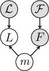

We define a distribution p(m) over matches, where a match m associates keypoints in the test image I and training images $$I_i$$

. We use kernel density estimation on translations proposed by all matches ${\mathcal M}_i$ between keypoints in the test image and those in the i-th training image. For a match $m \in {\mathcal M}_i$ , the probability p(m) expresses the translational consistency of the match m with respect to all other matches in ${\mathcal M}_i$ . This non-parametric representation accepts multi-modal distributions, where the keypoints in the upper abdomen may suggest a different transformation than those in the lower abdomen.

2.2 Keypoint Voting

After establishing matches for keypoints in the test image, we estimate an organ label L for each keypoint in the test image based on the generative model illustrated above. The latent variable m represents the keypoint matches found in the previous step. Keypoint labeling is helpful to obtain a coarse representation of the image, including rough location of organs. Additionally, we use the keypoint labels to guide the image segmentation as described in the next section. For inference of keypoint labels, we marginalize over the latent random variable m and use the factorization from the graphical model to obtain

$\begin{aligned} p(L, F, {\mathcal L}, {\mathcal F})&= \sum _{m \in {\mathcal M}(F)} p( L , F, {\mathcal L}, {\mathcal F}, m) \end{aligned}$

(3)

$\begin{aligned}&= \sum _{m \in {\mathcal M}(F)} p( L | {\mathcal L}, m) \cdot p(F | {\mathcal F}, m) \cdot p(m ), \end{aligned}$

(4)

where ${\mathcal M}(F)$ contains matches for keypoint F across all training images. The marginalization is computationally efficient, since we only compute and evaluate a sparse set of matches. We define the label likelihood

$\begin{aligned} p(L = l | {\mathcal L}, m ) = \left\{ \begin{array}{rl} 1 &{} \text{ if } {\mathcal L}_{m(F)} = l, \\ 0 &{} \text{ otherwise, } \end{array} \right. \end{aligned}$

(5)

where ${\mathcal L}_{m(F)}$ is the label of a training keypoint that the match m assigns to the test keypoint F. The keypoint likelihood is based on the descriptor of the keypoint

$\begin{aligned} p(F | {\mathcal F}, m) = \frac{1}{\sqrt{2\pi \tau ^2}} \exp \left( -\frac{ \Vert F^D - {\mathcal F}^D_{m(F)} \Vert _2^2}{2\tau ^2} \right) , \end{aligned}$