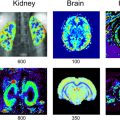
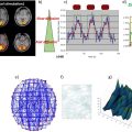
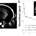
12.2.1.1. Signal-to-noise ratio and sensitivity

SNR is one of the most important parameters in MRI because its increase can be exploited to improve spatial (Figure 12.3) or temporal resolution. For fixed temporal and spatial resolutions, it provides better sensitivity, which is particularly beneficial for quantitative imaging.

According to theory, the SNR variation is supralinear as a function of the main magnetic field strength (Ocali and Atalar 1998). This has recently been confirmed by experimental measurements. Considering all of the parameters influencing the measurements for a range of B₀ between 1.5 and 9.4 T, the SNR was found to increase as B₀^1.65 (Pohmann et al. 2016). Thus, the expected gain in SNR when using 7 T instead of 3 T, assuming the same RF coil design, is approximately a factor of 3.1 (see Figure 12.4).

COMMENT ON FIGURE 12.4.– (a) SNR variation as a function of magnetic field B₀. Modified from Pohmann et al. (2016), with the authors’ permission. (b) Simulated variation of the ultimate SNR (a.u.) in gray matter (GM) and white matter (WM) as a function of the magnetic field. The dashed lines represent the linear extrapolation of uSNR at lower fields. Modified from Guérin et al. (2017), with the authors’ permission. The notion of ultimate SNR refers to the maximum theoretically possible SNR, regardless of the coil geometry (Ocali and Atalar 1998).

SNR is even more important in parallel imaging with SENSE- or GRAPPA-based reconstructions, which have been widely adopted to reduce the scan time at the price of decreased SNR (compared to conventional Cartesian-based MRI with a receive coil array). This reduction is dependent on the acceleration factor R and the geometry factor “g” related to coil geometry according to the formula SNR_R = SNR_0/(g.R^1/2) (Pruessmann et al. 2001). However, for a given coil design, it has been shown that, when B₀ increases, g has less influence on the result, thereby increasing the advantage of parallel imaging at ultra-high field (Wiesinger et al. 2004).

Finally, while MRI usually detects hydrogen nuclei (¹H), other nuclei (X) with a nonzero nuclear spin can also be used. Due to the concentration of the isotope in the human body and its gyromagnetic value, the observable signal is typically very low at conventional magnetic fields employed in clinics, leaving little room for alternative approaches. At 7 T, the SNR gain partially compensates for this weakness, thereby opening new perspectives for X-nuclei imaging and spectroscopy (see Chapter 9). The best candidates are in the order of decreasing available signal: ²³Na sodium, which can be used as a marker of tissue viability and the investigation of inflammatory and (neuro-)degenerative processes (Thulborn 2018), particularly through the measurement of the total sodium concentration (Burstein and Springer 2019); ³¹P phosphorus for investigating the energy metabolism and pH measurement (Liu et al. 2017); and ¹³C carbon. Lower-abundance ³⁹K potassium and ¹⁷O oxygen remain hardly detectable at 7 T. Finally, it should be noted that the low-sensitivity nuclei that are naturally absent in the human body can also be considered for 7 T imaging. This is the case of ⁷Li lithium used in psychiatry to evaluate the efficacy of some treatments (Stout et al. 2020).

12.2.1.2. Contrasts (BOLD/T₂*, T₁, etc.)

Besides the SNR and sensitivity, the contrast-to-noise ratio (CNR), measured from the difference in signal between two tissues, is also very important. High CNR can be useful for medical diagnosis in detecting small pathological anomalies or simply for the identification and delimitation of tissues from their intrinsic properties (T₁, T₂, T₂*). At 7 T, T₂* and T₁ contrasts can be particularly useful.

For a variation of the magnetic field (B) in a sample according to B = μ₀.(1+χ).B₀, with μ₀ as the vacuum permeability and χ as the magnetic susceptibility of the sample, the magnetic field non-uniformities at the interface between two tissues with different magnetic susceptibility properties (Δχ = χ₂ − χ₁) are given by ΔB∝Δχ.B₀. Therefore, increasing the magnetic field leads to linearly increased sensitivity to magnetic field inhomogeneities at the interface between compartments with different magnetic susceptibility. These variations of the local magnetic field, created at microscopic and mesoscopic scales (contributions to T₂) as well as at a macroscopic scale (γ.ΔB₀), perturb the transverse relaxation, leading to the so-called T₂* that satisfies the equation 1/T₂* = 1/T₂ + γ.ΔB₀ (van der Kolk et al. 2013). These perturbations imply greater sensitivity of T₂*-weighted sequences, such as gradient echo ones, at 7 T compared to conventional fields.

This sensitivity offers new perspectives, in particular for functional imaging (fMRI). fMRI is based on the variations of blood flow and volume, as well as deoxyhemoglobin concentration, during neuronal activation, which cause changes in magnetic susceptibility and, as a consequence, in signal (blood oxygenation level dependent (BOLD) effect (see Chapter 5)). Combined with a possible improvement of spatial resolution, ultra-high field fMRI (Yacoub and Wald 2018) becomes more sensitive and enables us to, for example, distinguish the activation within subcortical layers (Figure 12.5).

It should be noted that increasing the strength of the magnetic field causes additional distortions but also greater sensitivity to physiological noise (see section 12.2.2). As a result, the parameters of a functional imaging sequence should be selected to maintain the temporal SNR (tSNR) within the thermal noise regime (Triantafyllou et al. 2011) to fully benefit from the increased field.

The literature suggests that an advantage exists in using T₂ weighting rather than T₂* weighting at ultra-high magnetic fields. Indeed, T₂ weighting improves the specificity of the BOLD signal by strengthening the contribution of capillaries compared to the large vessels inside a voxel (Uludağ et al. 2009). However, in practice, T₂ weighting is rarely used because it requires spin-echo sequences that deposit a considerable amount of energy in the tissues, which limits their applications to small volumes of interest.

Susceptibility weighting imaging (SWI) (Haacke et al. 2004) and quantitative susceptibility mapping (QSM) (de Rochefort et al. 2010) methods also greatly benefit from higher magnetic fields. The most spectacular applications include vascular network imaging (venography) (Koopmans et al. 2008) (see Figure 12.6), imaging of deep brain structures (subthalamic nuclei, basal ganglia, etc.) (Abosch et al. 2010), or the visualization of the central vein in the context of multiple sclerosis (MS), as described in section 12.4.

Finally, some applications also benefit from the variation of the longitudinal relaxation time (T₁) with the magnetic field. In biological tissues, the value of T₁ increases with the field strength (Rooney et al. 2007; Rodgers et al. 2013). In its generalized form, the variation of T₁ is expressed as T₁ (s) ~ A.ν₀ ^B, with ν₀ as the resonance frequency (Hz) and A and B two tissue-dependent constants (Bottomley et al. 1987).

At first glance, this increase could be perceived as a disadvantage. For instance, in neuroradiology, distinguishing between gray and white matter can become more difficult on conventional T₁-weighted images. However, this increase can be exploited for vascular imaging with contrast injection (Hagberg and Scheffler 2013) and without contrast agents (time of flight (ToF)) (Kang et al. 2010). In fact, the relaxation times of the blood and contrast agents, such as gadolinium, are less affected by the increase in B₀ than the adjacent tissues (Zhang et al. 2013). Thanks to a better SNR, spatial resolution and efficacy in suppressing the background signal (von Morze et al. 2007), the difference between the blood (injected or not) and static tissues is amplified, providing a better demarcation of the arterial network and eventual extravasation toward surrounding tissues.

A longer T₁ is also advantageous for applications with longitudinal magnetization preparation before the image acquisition; an example consists of cardiac tagging (used for investigating myocardial contractions), whose efficacy is improved over several cardiac cycles thanks to the longer T₁ values at 7 T (Rodgers et al. 2013).

12.2.1.3. Spectral broadening (MRS, CEST, etc.)

The domains of metabolic imaging and magnetic resonance spectroscopy (MRS) benefit from increased magnetic fields as well. Both for single voxel applications (single voxel spectroscopy (SVS)) or for spectroscopic imaging (chemical shift imaging (CSI)), the increased SNR in MRS can be exploited to reduce the voxel size and, hence, the partial volume effects in order to make the acquired metabolic spectrum more specific to the investigated tissues (e.g. discrimination of neurochemical profiles within the thalamic nuclei (Donadieu et al. 2016)).

More importantly, the spectral resolution between two species (Δω) increases linearly with B₀ (according to Δω = γ·(σ₂ − σ₁)·B₀, with σ being the chemical shift of each of these two species), thus highlighting the contribution of proton populations that could not be previously distinguished, thereby improving both the sensitivity and specificity of the technique. To fully benefit from these advantages, a good uniformity of B₀ and B₁⁺ is required, together with the implementation of specific acquisition and post-processing strategies (adiabatic pulses, frequency stabilization, etc.) (Henning 2018).

Chemical exchange saturation transfer (CEST) (Ward et al. 2000; Kogan et al. 2013), which enables the indirect detection of metabolites or molecules containing protons that can be exchanged via magnetization transfer from the pool of bound protons to the pool of free protons, can also benefit from a higher magnetic field. In the human body, these metabolites include the amide protons (APT), glycosaminoglycans (gag), glycogen, glutamate (Glu), etc., which can be notably used to investigate tumors (APT-CEST) or the cartilage (gag-CEST), for example. Once again, higher SNR provides better sensitivity (Singh et al. 2012) and improved frequency separation is advantageous due to the possibility of distinguishing components that were so far hardly discernible from the water peak (e.g. hydroxyl protons, which have a chemical shift between 0.5 and 1.5 ppm). It should be noted that at 7 T, all of these CEST applications remain still largely challenged by the problems related to the non-uniformities of the static and radiofrequency fields.

12.2.2.1. B₀ inhomogeneity

The scanners are manufactured to provide certain hardware specifications of constant uniformity of the static magnetic field B₀ inside the MRI bore over a diameter of spherical volume (DSV), regardless of the system’s field (see Chapter 1). Introducing an object or a patient inside the bore causes local field inhomogeneities (Schenck 1996) that increase linearly with B₀.

This heterogeneity, in particular at the interfaces between media with different magnetic susceptibilities χ, can be partially corrected using shim coils installed in the gradient insert. However, even if significant improvements can be obtained locally, these non-uniformities cannot be always compensated; this is the case of bone/tissue interfaces in the spine, air/tissue in the nasal cavity or near the lungs, or in the presence of metallic implants. Depending on the type of sequences, these effects can translate into artifacts, distortions, and signal loss in the images, especially in non-Cartesian imaging sequences, EPI sequences used in functional and diffusion imaging, or in spectroscopy.

This problem can be addressed using more B₀ shim coils (third spherical harmonic orders), gradient coil inserts dedicated to the organ to be scanned (Stockmann and Wald 2018), or dynamic shim strategies for multislice acquisitions with a controlled current in the shim coils for each imaging slice (Sengupta et al. 2011).

It should be noted that the variations of the B₀ field due to breathing (variation of the lung volume and intrinsic susceptibility effects) can also be problematic at 7 T, in particular for EPI- or gradient echo-based imaging and spectroscopy. This phenomenon, called “dynamic variation of the B₀ field”, can induce a significant and penalizing signal attenuation. When imaging the spinal cord for instance, B₀ variations in the order of 70 Hz have been reported during the breathing cycle, associated with a signal loss between 40 and 120% (Vannesjo et al. 2019). In the brain, these fluctuations are lower, in the order of 10 Hz, but they are still present (Vannesjo et al. 2015).

12.2.2.2. Feasibility of ultra-high resolution imaging

Increasing the spatial resolution provided by 7 T is hindered by higher sensitivity to the patient’s motion (physiological or involuntary). Physiological movements are related to the cardiac rhythm, cerebrospinal fluid pulsations, as well as breathing, which cause dynamic variations of B₀ non-uniformities in addition to organ displacement. Synchronizing the MRI acquisition with the respiratory or cardiac cycle (via pressure or pulse sensors or ECG electrodes) remains necessary for cardiac, medullar or abdominal applications as conventionally performed at lower fields. Physiological data can also be recorded, such that they can be filtered or their influence uncorrelated during image post-processing (Lévy et al. 2021). It should be noted that the signal quality of the electrocardiogram at 7 T can be considerably perturbed inside the magnet by the magnetohydrodynamic effects of blood flow (Stäb et al. 2016).

Motion can also be related to patient compliance (Marrakchi-Kacem et al. 2016). For brain applications, dedicated devices have been developed to ensure the reliability and reproducibility of investigations with very high spatial resolution. These devices employ motion control systems based on optical cameras (Stucht et al. 2015; Mattern et al. 2018) or magnetic field cameras (Haeberlin et al. 2015) and involve a feedback loop that modifies in real-time the gradients applied by the imaging sequence to take into account the changes in the patient’s position. Furthermore, the information can be also used a posteriori to correct the motion effects during post-processing. Regardless of the approach, these methods are currently limited to research settings.

12.2.2.3. B₁⁺ non-uniformity

In terms of SNR and CNR, the benefit of MRI at 7 T mentioned in section 12.2.1 is neutralized by the inhomogeneous propagation of the radiofrequency field in the human body at this frequency. Maxwell equations governed by the electromagnetism laws show that when the resonance frequency is increased, the wavelength of the RF fields inside the tissues decreases down to the size of the body region to be scanned (between 10 and 15 cm, see Figure 12.7(a)), potentially with destructive interferences (Collins and Wang 2011) or dielectric artifacts (Hoult and Phil 2000) with conventional excitation approaches, depending on the coil geometry, scanned region and its relative permittivity ε_r and electrical conductivity σ. In practice, this translates into a modification of the B₁⁺ field within the tissues (nonuniform flip angle over the image, see Figures 12.7(f) and (g)), and consequently into spatial heterogeneities of the signal (signal loss artifacts) (see Figures 12.7(d) and (e)).

For scanners approved for clinical use, with currently authorized medical scans only in the brain and knee, radiofrequency heterogeneity in these anatomical regions remains overall limited and permits good diagnostic interpretation. Nevertheless, some precautions have to be taken in the frontotemporal regions and during quantitative imaging. To minimize these problems, other approaches are required: passive approaches based on dielectric pads, or active ones, based on imaging with parallel transmission (see section 12.5).

The non-uniformities of B₁⁺ field are also a limitation for all of the imaging sequences that exploit global inversions or saturations of the magnetization.

In quantitative imaging, such as CEST or T₁ relaxometry, the B₁⁺ heterogeneities have to be corrected to remove quantification biases (Kogan et al. 2013). Some sequences, such as the T₁-MP2RAGE (Marques et al. 2010), can be adapted to be relatively immune to B₁⁺ variations thanks to the type of employed RF pulses and a smart adjustment of the acquisition parameters (RF angles, inversion times, etc.).