Ultrasound Basics–Getting Started

This chapter is not a grueling review of the sometimes tedious physics of US but is a discussion of “how to”: turn on the machine, understand the US image, perform an examination, recognize and use US artifacts, and problem-solve when nothing seems to work. It is written to help the novice radiology resident deal with the sometimes terrifying nights on call alone in the hospital with surgeons hovering and the friendly sonographers at home in bed. The use and interpretation of Doppler US are covered in Chapter 11.

Getting Started

Surely the most basic, but commonly ignored, aspect of learning to perform an US examination is how to turn on the machine. A wide variety of US units made by many different manufacturers are in everyday use. For reasons forever unknown, the power-on switch is often wickedly hard to find. The beginning student of sonography should spend 30 minutes of initial training with an experienced sonographer reviewing machine start-up, patient data entry, image storage, the procedure for changing transducers, and basic “knobology” for all the US units you are likely to use. Your expertise is immediately suspect, by both patient and referring physician, if you need to spend 10 embarrassing minutes finding the “on” switch.

US examinations are routinely performed by placing the transducer on the patient’s skin. Because resistance to sound penetration is high at the skin surface, a sonolucent gel is used on the skin surface to promote sound transmission from the transducer into the patient through the skin. For patient comfort, the US gel should be kept warm in specially designed gel-warmers. For intracavitary US (transvaginal, transrectal), gel is placed on the transducer face. Then the transducer is covered with a sterile condom. The condom is in turn covered with additional sterile gel to promote sound transmission within the vagina or rectum. For intraoperative US, the exposed surgical bed is filled with sterile saline and the sterile condom-covered US probe can be placed directly on the structure of interest.

Understanding the US Image

The design of the transducer determines the shape and field of view of the US image. Basic transducer formats are sector, linear array, and curved array (Fig. 1.1) [1]. Sector transducers produce slice-of-pie-shaped images that are narrow in the near-field but have a wide view in the far-field. These transducers are optimal for examining larger organs from between the ribs. Vector transducers are basically sector transducers with the tip of the pie-slice-image cut off. Vector transducers provide slightly wider near field of view than do sector transducers. Linear array transducers produce rectangular images with width of the image determined by the physical width of the transducer face. Linear array transducers often offer the best overall image quality and are preferred for examining anatomy in the near-field, just beneath the skin surface. Curved array transducers are a cross between linear and sector transducers providing a broader view in the near-field while retaining a broad view in the far-field. The transducer face is wide and gently curved.

All US images are obtained by using a pulse-echo technique (Fig. 1.2). All US transducers are sound transmitters and receivers. A brief (microsecond) pencil-beam-shaped pulse of US energy is directed into the patient. The transducer then becomes a receiver for echoes reflected back to the transducer from along the directed path of the US beam. All sound reflections detected are assumed to originate from the original “line-of-sight” of the
transmitted beam. Sound reflections from directions other than the “line-of-sight” are either not detected or produce artifacts that impair image quality (Fig. 1.3). Dots (pixels) in the US image are placed along the “line-of-sight” according to the strength of each echo (brightness = sound intensity) and the time at which the echo is received. Depth is directly proportional to time of echo receipt. The US computer assumes that the speed of sound in tissue is a constant (1540 m/sec). Thus the depth of a sound reflector is determined by the time from pulse transmission to echo reception divided by two (allowing for the beam to go out and the echo to return).

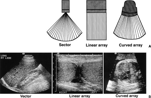Figure 1.1 Types of Ultrasound Transducers. Sector, linear array, and curved array transducers provide differing shapes in the ultrasound field-of-view. A. Note that the US beams from sector and curved array transducers diverge as they penetrate deeper into tissue. This divergence decreases lateral (perpendicular to the US beam) resolution compared to the linear array transducer. B. Sector transducers are optimal for imaging large structures deep in tissue, such as the kidney. The small face of the transducer allows imaging through the narrow sonographic window of the intercostal spaces. The diverging field of view allows visualization of the entire kidney. True sector transducers produce a “piece-of-pie” shaped image originating from a point source on the transducer face as shown in A. Vector transducers are sector transducers with the origin of the image on the transducer face widened slightly as in B. Linear array transducers are optimal for visualizing smaller structures, like the testes, breast, and thyroid, that are just beneath the skin. The wider field-of-view in the near field improves visualization of these superficial structures. Curved array transducers combine advantages of the sector and linear formats. These transducers are optimally used when the sonographic window is broad, such as in the second and third trimester of pregnancy.

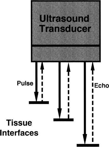Figure 1.2 Pulse-Echo Ultrasound. The US transducer sends a series of US beams into patient tissue. The US image is produced by the pattern of reflected beams (echoes) detected. All echoes are assumed to originate along the “line-of-sight” of the originally transmitted beam. The depth of an echo is determined by measuring the round trip time-of-flight from beam transmission to echo reception. Assuming that the speed of sound in human tissue is a constant 1540 m/sec, the depth of an echo can be accurately plotted on the resulting US image.

US transducers are designed to operate at a specified sound frequency. Medical ultra sound is performed using very high sound frequencies in the range of 1-20 MHz. The best image resolution is obtained by using the highest frequency possible. However, the higher frequencies are more limited in ability to penetrate tissue. Thus, lower frequencies are often used, accepting lower resolution as a trade-off for better penetration.

Images are displayed on a computer monitor. During the infancy of diagnostic US there was some controversy whether images should be displayed as “white on black” or “black on white.” White on black won. So virtually all gray-scale US imagesare displayed as tiny white dots on a black background (Fig. 1.4). Transverse images are routinely displayed with the
patient’s right side on the left side of the image as if we are examining the patient’s cross-section anatomy from below looking upward toward the patient’s head. This image display matches the convention for display of CT and MR images. Longitudinal images are displayed with the cranial aspect of the patient’s anatomy at the left side of the image.

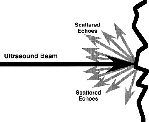Figure 1.3 Ultrasound Scatter. As the US beam passes through tissue, it encounters irregular reflecting surfaces that scatter echoes in many directions. Only the echoes that return to the transducer at the site of origin of the US beam are displayed on the image. Progressive scattering of the echoes attenuates the sound beam as it passes deeper into tissues. Scattering of the echoes also degrades the US image and produces artifacts by multipath reflection.

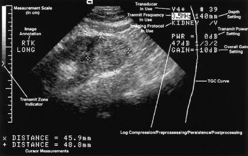Figure 1.4 Ultrasound Image Annotation. This image is produced on an Acuson (Acuson Medical Ultrasound Company, Mountain View, CA) US unit and also shows the typical image annotation of technical settings used to produce the image. The nature of each annotation is indicated in small print. Other manufacturers have similar technical annotations. The image shows a renal cell carcinoma (between cursors, +, x) arising from the right kidney.

How to Scan

When first encountering a modern computerized US unit, any novice will be impressed with the number of knobs, switches, track balls, display screens, and gadgets to be used and mastered. To simplify the process and diminish the intimidation factor, I suggest the beginner concentrate on finding and using only the following, much reduced, list of controls. Concentrate on your scanning technique and optimize the use of these controls. Depend upon experienced sonographers to help you with the fine-tuning that produces the dramatic images in the “sonogenic” patient or saves the study in the nearly impossible-to-image patient.

The Knobs

Depth

The depth knob controls the deep portion of the field of view of the US image. As shown in Figure 1.4, the depth setting of 140 mm indicates the distance in the patient from the transducer face on the patient’s skin to the curved bottom of the image. Depth should be adjusted to match the anatomy under inspection. Depth set too deep will minify the image, cramming the useful information into the top part of the image and wasting the bottom portion of the image. Depth set too superficial will fail to display the entirety of larger organs. You won’t know where you are. Depth should be adjusted constantly to show the structure of interest and to optimize resolution (Fig. 1.5).

RES

RES (Resolution Expansion Selection) is another form of depth control. When the RES knob is pushed a RES box is displayed on the image (Fig. 1.6). Additional controls allow the operator to adjust the location and size of the RES box. When the RES knob is pressed a second time the image within the RES box is magnified to occupy the full image display. RES is useful for displaying and measuring small structures such as the common bile duct in the porta hepatis. RES is an Acuson (Acuson Medical Ultrasound Company, Mountain View, CA) trademark function. Other US manufacturers have similar functions identified by a variety of different names.

Gain

Gain is the US term for amplification. The intensity of returning echoes is amplified to produce a pleasing image. Gain is similar to the volume control on a stereo music system. Turn
gain up to produce an overall brighter image. Turn gain down to produce a darker image. Too much gain will display false echoes in cystic structures and make them appear complex or solid. Too little gain may make solid lesions appear cystic. One knob controls overall gain of the entire image. An array of time-gain-compensation (TGC) knobs controls gain at various depths in the image.

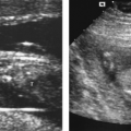
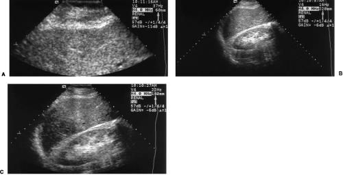Figure 1.5 Depth Settings. A. Depth set too shallow (60 mm-arrow) shows an image with anatomy that is difficult to recognize. B. Depth set too deep (220 mm-arrow) wastes a large portion of the field of view and minifies the image. C. Depth set appropriately (140 mm-arrow) shows the liver and kidney in appropriate perspective.

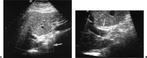Figure 1.6 Resolution Expansion Selection (RES) Function. A. Image of the liver shows the porta hepatis. The portal vein and common bile duct are small structures, and their visualization is limited. The operator has placed a RES box (arrow) around the portion of the image to be magnified with improved resolution. B. By pressing the RES button a second time, the RES function is activated, and the anatomy of interest fills the image. Larger image size allows more accurate measurement of this normal common bile duct (arrow).

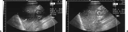Figure 1.7 Faulty Adjustment of Time-Gain-Compensation (TGC) Curve. A. Image through the liver shows a central band of dark echoes (curved arrow) caused by faulty adjustment of the TGC curve (short arrow) . B. Proper adjustment of the TGC curve (short arrow) produces a uniform appearance to the liver. Note that image resolution is the best at the level of the transmit zone (long arrow) .

Time-Gain-Compensation

As the US beam travels deeper in tissue, its intensity is progressively attenuated by tissue absorption of sound energy and by scattering of the beam in different directions by tissue interaction. To compensate for this loss of sound energy, the returning echoes are progressively amplified proportional to the time of their return to the transducer. Echoes from deeper in the tissue return later to the transducer and are amplified to a greater degree. This method of amplification is called time-gain-compensation.

The controls for TGC are a series of sliding knobs corresponding to depth in the image. Gain can be individually adjusted for multiple levels of depth. The resulting TGC curve is often displayed on the side of the US image. The knobs should be aligned in an even curve that produces a pleasing image (Fig. 1.7).

Transmit Zone

Transmit zone is an operator-adjustable, transmit-focus function that allows for additional image enhancement of the structures adjacent to the transmit zone marker. The transmit zone marker should be set at, or just below, the structure of greatest interest (Figs. 1.7, 1.8). When no moving structures are within the field of view, multiple transmit zones can be used to improve quality of the entire image (Fig. 1.1B).

Freeze and Store

US examination is a dynamic process that allows viewing of enough frames of information per second to be considered “real-time.” Just as in a movie, the “real-time” image is actually made up of numerous individual frames or “snapshots.” These are captured and displayed quickly enough to evaluate motion of the beating heart, the moving diaphragm, or the pulsating aorta. To view and record individual images, press the FREEZE button. To store the image for viewing later and to create a permanent image file of the examination, press the STORE button. A CINE function is usually available to review and store recent images, just in case your finger is too slow hitting the FREEZE button.

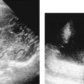
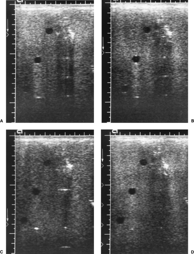Figure 1.8 Effect of Transmit Zone Focusing Shown on an Ultrasound Phantom. US phantoms are used to quality control US equipment. This tissue-equivalent phantom simulates three cysts at different depths in tissue. In A, the transmit zone (arrow) is set at a superficial depth. The upper and middle cysts are well seen, but the deepest cyst is barely visible. In B, the transmit zone (arrow) is set at the level of the middle cyst. Now the deepest cyst is seen but not well characterized. In C, the transmit zone (arrow) is set at the level of the deepest cyst, providing a quality image of it, but a poor image of the most superficial cyst. In D, multiple transmit zones (arrow) are used to provide a quality image of all three cysts. Multiple transmit zones are effectively used whenever there is little or no motion of the imaged structures.

Scan Technique

The physician sonologist has the opportunity to combine clinical diagnosis with sonographic examination. Any pertinent previous imaging studies should be reviewed and correlated with the current clinical problem. The examining physician should query the patient regarding current symptoms and past medical history, especially noting any previous surgical procedures. Suspected masses can be evaluated by physical examination as well as by sonography. Focal areas of pain or tenderness can be examined dynamically and correlated with the US images.

Table 1.1. Choosing a Transducer

Examination	Recommended Transducer
Abdomen	2.5-4.0-MHz sector or vector
Kidneys and bladder	Harmonics often provide the best images
Gastrointestinal tract
Liver and renal transplants
Pelvis
Obstetric first trimester
Transabdominal	2.5-4.0-MHz sector or vector
Transvaginal	4.0-8.0-MHz curved or sector intracavitary
Superficial parts	7.0-10.0-MHz linear array
Scrotum
Thyroid
Breast
Extremity
Chest	5.0-7.5-MHz linear array for superficial pleural space
	3.5-4.0-MHz sector or vector
Neonatal brain	5.0-7.0-MHz sector
Obstetric second/third trimester	3.5-5.0-MHz curved array or
	3.5-5.0-MHz wide linear array
Prostate	4.0-8.0-MHz curved or sector intracavitary

The first step in US examination is to select the transducer most appropriate for the examination at hand (Fig. 1.1). Experience makes this selection easy. Table 1.1 provides some suggestions for the novice. Make sure the patient’s name and medical record number are entered into the US unit’s database to properly identify the examination. Position the patient appropriately for the examination to be performed. Explain what you are doing and why. Make sure the US gel is warmed and use it to cover the area of examination.

Wear examination gloves for any intracavitary examination or examination around open wounds or with broken skin. Many sonographers wear gloves for all examinations. Hold the transducer firmly with your thumb against the ridge or groove that marks the orientation of the transducer. This marker should always be directed toward the patient’s right side or toward the patient’s head to properly orient the image. Place the edge of your hand against the patient’s skin to stabilize the transducer and allow you to make fine gentle movements of the transducer. Begin scanning in an area where you think that recognizable anatomy should be. For example, start in the right upper quadrant of the abdomen to find the liver. Adjust the controls to fill the image with the anatomy of interest. Orient yourself to the three-dimensional anatomy of the patient. Move the transducer slowly to identify additional structures. The transducer can be moved freely in many directions to change the anatomy displayed. Don’t bounce around but stay focused in one area and use small adjustments. You can slide the transducer right or left, craniad or caudad. You can angle the transducer up or down. You can turn the transducer into transverse, longitudinal, or oblique orientations [2].

Only gold members can continue reading. Log In or Register to continue