Fig. 11.1
Normal trileaflet aortic valve in parasternal long-axis view (a) and parasternal short-axis view (b). Severe calcific aortic valve disease is shown at the bottom panels (c, d) from the same views. Arrows point to aortic valve leaflets which are thin and have wide systolic opening in the normal valve but are heavily calcified with restricted systolic opening in advanced disease. Also evident is the increased left ventricular thickness in the parasternal view (c) compared to a patient with a normal aortic valve (a)
Rotating the transducer clockwise approximately 90° will image the parasternal short axis. The transducer angle should be adjusted to the aortic valve level to view the aortic cusps in the center of the image. From this view all three leaflets can be identified as well as congenital abnormalities such as a bicuspid valve. Normal valves should appear thin and open freely into a circular orifice during systole. In CAVD, calcification of the individual leaflets and annulus can be identified as well as valve thickening or reduced systolic opening. A bicuspid valve can be identified by demonstrating only two leaflets during systole; frequently a prominent raphe can make distinction of a bicuspid from tricuspid valve difficult during diastole when the valve is closed and calcified. Other distinctive features for a congenital bicuspid valve may include systolic doming, elliptical-shaped systolic orifice, and a central to commissural opening pattern. A bicuspid valve is found in approximately 1 % of the general population as reported in autopsy and echocardiographic series, but the prevalence is higher in those with other congenital abnormalities such as Turner syndrome or coarctation of the aorta. Rheumatic disease can lead to aortic stenosis but is a distinct pathological process. Distinct echocardiographic features of rheumatic disease include commissural fusion and mitral valve involvement.
When transthoracic image quality is too poor to identify the etiology of the aortic valve disease, a transesophageal echocardiogram (TEE) can be performed. TEE provides higher resolution imaging than TTE, and images of the aortic valve can be obtained almost universally. However, TEE is a second-line choice for echocardiographic imaging in most situations as it carries procedural risk due to probe insertion into the esophagus and conscious sedation. The aortic valve can be imaged in long-axis and short-axis views from a high esophageal probe position at about 120° and 45° of rotation angle, respectively. The improved imaging resolution can help identify the correct number of aortic cusps, the anatomic orifice area at the leaflet tips, or any associated subvalvular or aortic root anomalies not identified by TTE. TEE imaging also allows 3D imaging of the valve which is helpful in distinguishing a bicuspid from a trileaflet valve (Fig. 11.2).
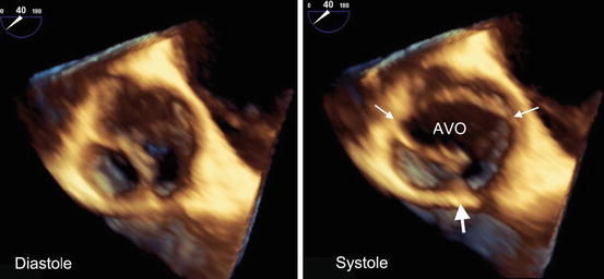
Fig. 11.2
A 3D TEE view from the aortic side of the valve appears tricuspid in diastole (a) but can be diagnosed as bicuspid in systole (b) with an oval aortic valve orifice (AVO) and two commissures (thin arrows) and a prominent raphe (thick arrow)
11.2.2 Velocity and Pressure Gradients
Doppler echocardiography allows measurement of various hemodynamic parameters that are important for the evaluation of CAVD severity (Table 11.1). By measuring backscatter ultrasound frequency changes due to movement of red blood cells, blood flow velocity can be accurately measured using the Doppler equation [1]. Normal aortic transvalvular blood flow is laminar and unobstructed with a peak aortic jet velocity (Vmax) between 1 and 2 m/s. In CAVD, as the aortic valve orifice narrows, the peak aortic velocity increases. Measuring Vmax requires a continuous-wave (CW) Doppler probe that is parallel to the direction of blood flow. Recorded velocities are displayed as a velocity curve with velocity on the vertical axis over time on the horizontal axis. In CAVD, irregular opening of the valve can lead to an unpredictable direction of the maximum blood flow velocity; thus, a thorough TTE Doppler evaluation requires searching for the highest velocity in multiple acoustic windows from the apical, parasternal, subcostal, and suprasternal transducer positions. TEE probe positions are constrained, and thus measuring aortic velocities can be frequently underestimated from misalignment.
Table 11.1
Calcific aortic valve disease echocardiographic measurements
Strengths | Weaknesses | |
|---|---|---|
Peak aortic jet velocity | Easy to measure | Underestimates severity in low-flow states |
Strongly associated with outcomes | Overestimate severity if significant pressure recovery | |
Mean gradient | Same as peak aortic jet velocity | Same as peak aortic jet velocity |
Effective aortic valve area (continuity equation) | Well validated with catheter-based valve areas | Highly dependent on LVOT diameter measurements |
Less flow dependent than peak velocity or mean gradient | Severity can be overestimated in significantly impaired flow states | |
Anatomic aortic valve area (planimetry) | Does not require Doppler echocardiography | Calcification limits visualization of anatomic orifice |
Irregular 3D orifice areas can lead to over- or underestimation on 2D imaging | ||
Not as well studied as effective aortic valve area for CAVD outcomes | ||
Velocity ratio | Simple to measure | Not validated with clinical outcomes |
Indirectly accounts for body size | May under- or overestimate severity with incorrect LVOT sample placement | |
Does not require measurement of LVOT diameter | ||
Valvuloarterial impedance | Global assessment of ventricular load | Requires multiple measurements to calculate compounding potential measurement errors |
Accounts for hypertension and stroke volume | ||
Energy loss index | Accounts for pressure recovery | Requires multiple measurements |
Improved severity estimation with small body types | Indexing to body surface area can overestimate severity in large body types | |
Less flow dependent than peak velocity and mean gradient | Severity can be overestimated in significantly impaired flow states | |
Valve calcification | Does not require Doppler | Mostly qualitative assessment |
Strongly associated with valvular outcomes | Weakly correlates with hemodynamics |
Under certain assumptions that are generally met in the clinical setting, instantaneous transvalvular pressure gradients (∆P) can be estimated from measured aortic jet velocities (v) using the simplified Bernoulli equation, ΔP = 4v2. A mean gradient can be obtained easily with commercial echo packages by averaging the instantaneous gradients over the duration of the systolic ejection period. Mean gradients calculated by Doppler measurements have been shown to have strong correlation with mean gradients obtained during catheterization [2, 3].
Transaortic valve velocity and pressure gradients can determine the presence of hemodynamically important aortic stenosis and categorize the severity into mild, moderate, or severe [4]. Although these parameters are easily measured with good reproducibility, there are potential pitfalls with measurement and interpretation that need to be avoided. First, optimal Doppler measurements require the intercept angle of the ultrasound beam to be as parallel as possible to the direction of blood flow. Nonparallel alignment will lead to underestimation of the velocity and pressure gradient. Measurements should be averaged over at least 3 beats in sinus rhythm and more if in an irregular rhythm; care should be taken to avoid measurement of post-extrasystolic beats. Assumptions of the simplified Bernoulli equation may not be met if there are very high velocities present in the left ventricular outflow tract (>1.5 m/s) or abnormalities of blood viscosity from profound anemia or polycythemia. Finally, velocity and pressure gradients are heavily flow-dependent measures. To avoid erroneous CAVD severity assessment, a high or low transaortic flow state and aortic valve area (AVA) need to be assessed.
11.2.3 Aortic Valve Area
The AVA can be estimated using the continuity equation which states that stroke volume through the left ventricular outflow tract (LVOT) is the same as the stroke volume through the aortic valve, SVLVOT = SVAV. Proximal to the stenotic valve, blood flow is laminar which allows calculation of stroke volume as SV = CSA × VTI, where CSA is the cross-sectional area of the flow and VTI is the velocity-time integral (area under the velocity curve). Substituting and rearranging the above equations provides the formula AVA = (CSALVOT × VTILVOT)/VTIAo. A simplified continuity equation substituting peak velocity (V) for VTI can be applied, AVA = (CSALVOT × VLVOT)/Vmax, because the shape and timing of the outflow tract and aortic jet velocity curves are similar. The cross-sectional area of the LVOT can be approximated from a zoomed in 2D TTE parasternal long-axis view. The diameter (D) of the LVOT is measured during mid-systole from the inner edge of the septal myocardium to the inner edge of the anterior mitral leaflet at the aortic cusp insertion points (Fig. 11.3a). By assuming a circular LVOT, the CSALVOT = π(D/2)2. This is an adequate assumption for stroke volume calculation with numerous studies validating continuity equation valve area with catheter-based valve area [5–7]. However, the actual LVOT is frequently more oval than round, which is important to account for in transcatheter aortic valve replacement (TAVR) which relies on 3D imaging measurements, either by computed tomography (CT) or TEE, of area and eccentricity to minimize complications [8].
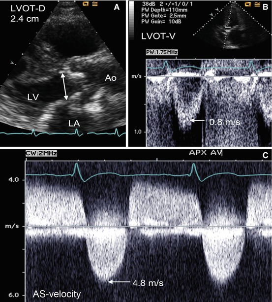
Fig. 11.3
Measurement of aortic valve area (AVA) in a patient with severe aortic stenosis. The left ventricular outflow tract (LVOT) dimension measuring 2.4 cm in a zoomed parasternal long-axis view (Panel A). Pulsed-wave Doppler shows a peak LVOT velocity of 0.8 m/s (Panel B), and continuous-wave Doppler through the aortic valve reveals a Vmax of 4.8 m/s (Panel C). The aortic valve area is severely reduced at 0.75 cm2 using the simplified continuity equation
Measurement of the peak velocities and VTI requires that the Doppler beam have a parallel alignment with the blood flow. This is achieved with the transducer in the apical position. To obtain the velocity curve at a specific location such as the LVOT, a pulsed-wave (PW) Doppler signal is needed. The PW Doppler allows placement of a sample volume on the ventricular side of the aortic valve at the same location where the LVOT diameter is measured. Velocities are recorded over time at the location of the sample volume, and velocity curves are produced on the spectral Doppler display. The VLVOT and VTILVOT are measured by tracing the modal velocity (brightest or most dense) portion of the spectral tracing (Fig. 11.3b) [1]. The Vmax and VTIAo through the aortic valve are measured from tracing the outer edge of the velocity curve from the maximum aortic jet obtained from the CW Doppler (Fig. 11.3c). Gain should be adjusted to produce a dark envelope around the spectral velocity curve with careful attention to avoid measuring the faint signal broadening produced from the transit-time effect of the ultrasound signal.
Alternative echocardiographic approaches can be used to estimate valve area when the continuity equation AVA appears discrepant to clinical findings or the above parameters cannot be obtained due to poor image quality. Planimetry in a short-axis view to measure the anatomic (geometric) orifice area can be performed [9, 10]. This can be limited if using 2D TTE due to difficulty obtaining an accurate planar image of an irregular 3D valve orifice. Additionally, poor image resolution and calcification artifacts can lead to inaccurate tracing of the valve area. When TTE quality is suboptimal, a TEE can be used to measure the LVOT diameter from a high esophageal probe position angled between 120 and 150°. The high-resolution and multiplane imaging capability of TEE also allows for improved planimetry of the valve area [11] but can still suffer from similar difficult visualization problems in advanced CAVD [12]. The anatomic valve area when correctly measured from planimetry is expected to be slightly larger than the effective orifice area calculated from the continuity equation due to contraction of the flow stream through a narrowing orifice [13].
New advances in 3D echocardiography may improve valve area estimation by overcoming some inherent limitations of 2D imaging. Improved planimetry has been demonstrated by allowing accurate determination of the narrowest valve plane to measure and has shown good correlation with Doppler-derived and catheter-derived valve areas (Fig. 11.4) [14]. 3D echocardiography may also produce a more accurate estimation of stroke volume from either directly measuring LVOT area [15], using real-time 3D ventricular volumes [16], or calculating color Doppler flow-volume curves [17]. Despite initial studies showing promise of 3D techniques improving AVA estimation, 2D Doppler-based continuity equation remains the echo gold standard until further studies demonstrate that 3D techniques are clinically reproducible and are associated with outcomes.
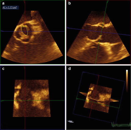
Fig. 11.4
Planimetry of the anatomic orifice valve area of a bicuspid valve using 3D echocardiography. Correct position at the leaflet tips in the transverse view (a) can be confirmed with 3D imaging by simultaneously viewing the perpendicular sagittal (b) and coronal (c) plane views. Note the systolic doming of the bicuspid valve in the long-axis (sagittal plane) view (b)
11.2.4 Additional Measurements of Hemodynamic Severity
Traditional markers of hemodynamic severity (peak aortic jet velocity, mean gradient, and aortic valve area) may not always correlate with each other, clinical symptoms, left ventricular function, or outcomes. To resolve discrepancies, additional severity indices have been suggested that may help improve CAVD classification. A simple measure is the velocity ratio (or dimensionless index) defined as VLVOT/Vmax, where VLVOT is the peak velocity obtained in the LVOT from the PW Doppler and Vmax is the peak aortic jet velocity as described in the previous sections. The ratio avoids errors in the LVOT area estimation which may be significant due to the LVOT diameter measurement being squared in the area equation.
In small individuals, the indexed AVA may be appropriate to use, AVA/body surface area (BSA), as a person with a small body type (height <135 cm, BSA<1.5 m2, body mass index (BMI) <22) may have a small but normal LVOT, AVA, and aorta. Indexing the valve area may reclassify smaller individuals from severe to moderate aortic stenosis (AS), but indexing all patients, particularly with extreme obesity, can lead to substantial overestimation of severity and should not be relied upon [18].
Another issue common to small body types and aortas is the concept of pressure recovery, the reconversion of kinetic energy into potential energy leading to an increase of pressure downstream from a stenosis. Doppler-derived pressure gradients represent the difference between left ventricular pressure and pressure in the vena contracta (lowest pressure in a stenosis), but do not measure the pressure recovery phenomena captured by a catheterization-based gradient (net pressure gradient). Pressure recovery accounts for differences between catheter- and Doppler-derived data [19, 20]. The net pressure gradient better reflects the hemodynamic significance and the amount of energy loss by the stenosis. To account for pressure recovery using echocardiography, Garcia and colleagues developed and validated the energy loss index (ELI) = [EOA × Aa/(Aa–EOA)]/BSA, where EOA is the effective orifice area using the Doppler-based continuity equation valve area and Aa represents the cross-sectional area of the aorta measured at 1 cm downstream of the sinotubular junction [21]. The ELI can be considered in situations when pressure recovery may be significant, such as individuals with aortic diameters <3 cm. The ELI has been shown to reclassify CAVD severity and provide independent and prognostic information above traditional severity measures [22, 23].
Hypertension is common in CAVD and can adversely affect hemodynamics, symptom burden, and traditional echo measure assessment [24–26]. To account for the “double load” of hypertension and aortic stenosis on the left ventricle, calculation of the valvuloarterial impedance (Zva) can be obtained using the equation Zva = (SBP + MGnet)/SVi, where SBP is the systolic blood pressure, MGnet is the mean net pressure gradient (taking into account pressure recovery), and SVi is the stroke volume indexed for BSA [27]. This global measure of vascular, valvular, and ventricular interplay may improve risk stratification in patients with asymptomatic moderate to severe CAVD [28].
11.3 Echocardiography and CAVD Outcomes
11.3.1 Aortic Valve Sclerosis and Cardiovascular Outcomes
Evidence of early CAVD, aortic valve sclerosis (AVS), can be detected by echocardiography as thickening and calcification of the aortic valve without obstruction to left ventricular outflow. The precise definition of AVS in clinical studies has varied using different qualitative descriptions of thickening, calcification, and cutoffs for hemodynamic significance. This lack of uniformity can lead to interobserver variability for diagnosing AVS between echocardiographers in the clinical setting [29]. Additionally, instrument settings can alter the interpretation of aortic valve thickening. The use of tissue harmonic over fundamental imaging has been demonstrated to significantly increase the diagnosis and severity of AVS [30]. Calcification of the aortic valve leaflets appears as bright focal echodensities and is most often qualitatively graded as mild (small isolated spots), moderate (multiple larger spots), or severe (extensive involving all cusps). In an effort to quantify valve thickening and calcification, measurement of ultrasound backscatter amplitude from aortic valves has demonstrated feasibility and reproducibility in animal models and small samples of elderly volunteers [31–33]. However, the value of backscatter quantification over qualitative assessment in longitudinal studies has yet to be evaluated and is not practiced in clinical settings.
Despite the potential heterogeneity of diagnosis, AVS has consistently been associated with cardiovascular outcomes. Whether the increased risk is due in part to a direct mechanistic effect from CAVD or only a marker of cardiovascular disease remains unresolved. CAVD is a progressive condition and longitudinal echocardiographic studies have shown AVS progression to hemodynamically significant AS. In a study of 400 subjects with AVS by Faggiano et al. [34], 33 % developed some degree of AS over a mean follow-up of 44 months. In the subgroup with over 5 years of follow-up, 22 % advanced to either moderate or severe AS. In a larger confirmatory study by Cosmi et al. [35], 2,131 patients diagnosed with valve thickening that had serial echocardiograms were evaluated for hemodynamic progression. These investigators found that 5.4 % of their AVS patients advanced to moderate or severe AS over a mean of 7.4 years; mitral annular calcification was the only identified risk factor for progression in multivariable modeling. Similarly, in an elderly population-based cohort in the Cardiovascular Health Study, 9 % of the 1,610 participants with baseline AVS developed AS over a 5-year period [36].
The association of early CAVD with the short-term risk of cardiovascular outcomes cannot be fully explained from the relatively slow progression to hemodynamically significant AS. Multiple echo studies have identified similar cardiovascular risk factors between coronary artery disease (CAD) and CAVD, including age, male sex, hypertension, diabetes, low-density lipoprotein cholesterol, and smoking [37–40]. In Cardiovascular Health Study participants with baseline AVS and no known CAD, cardiovascular death risk was increased by 52 % and myocardial infarction risk by 40 %, even after adjustment for traditional cardiovascular risk factors [41]. Subsequent studies have attributed some of the increased risk to concomitant CAD and inflammation [42, 43].
11.3.2 Aortic Stenosis and Valvular Outcomes
In patients with hemodynamically significant CAVD, progression to symptoms, aortic valve replacement (AVR), and death have been studied by several approaches. The natural history of aortic stenosis was first defined in autopsy series prior to the use of echocardiography [44]. These initial series described a long latent asymptomatic phase of disease that would eventually lead to symptoms (angina pectoris, syncope, and heart failure) which herald a poor prognosis. Over 75 years later, the prognosis of uncorrected symptomatic severe aortic stenosis remains dismal with a reported 68 % mortality over 2 years [45]. AVR is currently the only intervention known to reduce adverse clinical outcomes in symptomatic severe AS.
Echocardiographic studies have established predictors of clinical outcomes in patients with asymptomatic aortic stenosis (Table 11.2). Hemodynamic severity by TTE is the cornerstone of predicting valvular outcomes in AS. Vmax is most consistently associated with outcomes across longitudinal studies after adjusting for clinical and echocardiographic parameters, including mean gradient and valve area [28, 46–49]. Those with Vmax >4 m/s have up to 80 % likelihood of AVR or death over the next 2 years [47]. Additionally, moderate to severe calcification of the aortic valve by TTE has been shown to be a strong predictor of AVR and death in mild, moderate, and severe AS [50, 51]. The prognostic value of calcification becomes attenuated in hemodynamically very severe AS (Vmax ≥5 m/s) as it almost universally presents and because progression to symptom onset is rapid in all patients with this degree of valve obstruction (Fig. 11.5) [52]. The combination of rapid hemodynamic progression (increase in Vmax ≥0.3 m/s/year) and significant valve calcification can identify a very high-risk cohort.
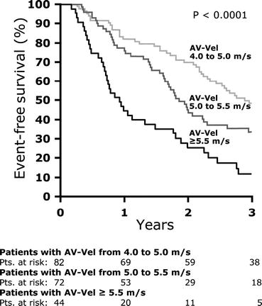
Table 11.2
Echocardiographic predictors of calcific aortic valve disease outcomes
Study | Year | N | Follow-upa (months) | Echo measurement | Outcome | Results |
|---|---|---|---|---|---|---|
Pellikka [46] | 1990 | 143 | 21 | Vmax ≥4.5 m/s | AVR or cardiac death | RR 4.9 (95 % CI, 1.64–14.6; p = 0.004) |
Otto [47] | 1997 | 123 | 30 | Vmax | AVR or death | Categorized event rates at 2 years of 79 % (>4 m/s), 34 % (3–4 m/s), and 16 % (<3 m/s); p < 0.001 |
Rosenhek [50] | 2000 | 128 | 22 | Calcification score (3 or 4) | AVR or death | RR 4.6 (95 % CI, 1.6–14; p < 0.01) |
Rosenhek [51] | 2004 | 176 | 48 | Vmax ≥3 m/s calcification score (3 or 4) | AVR or death | RR 1.6 (95 % CI, 1.04–2.8; p = 0.034) |
RR 2.0 (95 % CI, 1.3–3.3; p = 0.0012) | ||||||
Pellikka [48] | 2005 | 622 | 65 | AVA (per 0.2 cm2) | Symptoms | RR 1.26 (95 % CI, 1.08–1.47; p = 0.004) |
Vmax (per 1 m/s) | AVR or cardiac death | RR 1.20 (95 % CI, 1.06–1.36; p = 0.006) | ||||
All-cause mortality | RR 1.46 (95 % CI, 1.03–2.08; p = 0.03) | |||||
Hachicha [54] | 2009 | 544 | 30 | Zva (per mmHg∙ml/m2) | Death | RR 1.36 (95 % CI, 1.03–5.75; p = 0.03) |
LVH | RR 1.66 (95 % CI, 1.01–2.73; p = 0.05) | |||||
Rosenhek [52] | 2010 | 116 | 41 | Vmax ≥5.5 m/s | AVR or cardiac death | RR 1.88 (95 % CI, 1.19–2.96; p = 0.007) |
Lancellotti [28] | 2010 | 163 | 20 | Vmax (per 1 m/s) | Symptoms, AVR, or death | RR 1.6 (95 % CI, 1.01–2.5; p = 0.04) |
Zva (per mmHg∙ml/m2) | RR 1.6 (95 % CI, 1.25–2.0; p = 0.001) | |||||
GLS (per 1 %) | RR 1.1 (95 % CI, 1.01–1.2; p = 0.03) | |||||
Stewart [49] | 2010 | 183 | 31 | Vmax (per 0.5 m/s) | Symptoms | RR 1.43 (95 % CI, 1.25–1.64; p < 0.0001) |
AVA (per 0.1 cm2) | RR 1.13 (95 % CI, 1.05–1.22; p 0.04) | |||||
Rieck [53] | 2012 | 1418 | 43 | Zva >5 mmHg∙ml/m2 | AVR, CHF hospitalization, or death | RR 1.41 (95 % CI, 1.12–1.78; p = 0.004) |
Bahlmann [23] | 2013 | 1563 | 51 | ELI (per cm2/m2) | AVR, CHF hospitalization, or death | RR 2.05 (95 % CI, 1.48–2.85; p < 0.001) |
Fig. 11.5
Event-free survival in patients with severe aortic stenosis stratified by peak aortic jet velocity (Vmax) (Rosenhek et al. [52])
Newer echocardiographic measures of hemodynamic severity, ELI and Zva, also have been evaluated in longitudinal outcome studies [23, 28, 53, 54]. In a large subcohort of the Simvastatin and Ezetimibe in Aortic Stenosis (SEAS) study, ELI provided independent prognostic information beyond Vmax and mean gradients [23]. However the discriminatory ability of ELI for aortic valve events was similar to AVA, and both perform less well than the Vmax. In the same SEAS study population, a high Zva was found to be predictive for aortic valve events independent of Vmax and mean gradient, but was no longer significant when adjusting for AVA [53]. Despite the logical hemodynamic basis for these measures, their ability to associate with CAVD outcomes independent of traditional measures has yet to be proven. Future studies validating these measures with outcomes when traditional measures and clinical findings are discrepant may prove useful [55].
11.4 CAVD Pathophysiology and Echocardiography
11.4.1 Ventricular Changes
11.4.1.1 Hypertrophy
In advancing CAVD, valvular obstruction to left ventricular (LV) outflow leads to significant afterload excess. In most patients, pumping function is preserved and wall stress remains normal with a ventricular “response” to pressure overload of hypertrophy and concentric remodeling. These changes have been thought to be “compensatory” in the past but may instead be part of the disease process leading to myocardial fibrosis and persistent diastolic dysfunction even after AVR. Changes in ventricular size and geometry can be assessed with standard parasternal 2D TTE and M-mode imaging, although 3D ventricular volumes are more accurate and reproducible and are likely to replace linear and 2D measurements in the near future.
The most utilized measurements are end-diastolic minor-axis linear dimensions of septal (SWTd) and posterior wall thickness (PWTd) and LV cavity (LVIDd). Measurements should be obtained by 2D directed M-mode perpendicular to the LV long axis at the tips of the mitral leaflets [56]. If the M-mode beam cannot be aligned appropriately, 2D measurements may be used although the lower frame rate limits identification of the endocardial border. From these measurements, LV mass can be estimated from the following validated formula:LV mass = 0.8 × {1.04[(LVIDd + PWTd + SWTd)3–LVIDd3]} + 0.6g [57]. Cutoff values for hypertrophy are gender specific and indexed by BSA, 95 g/m2 for women and 115 g/m2 for men. Changes in LV geometry can be described as concentric when regional wall thickness (RWT) exceeds 0.42, using the formula RWT = (2 × PWTd)/LVIDd.
Related posts:
 Molecular Imaging of Macrophages in Atherosclerosis
 Molecular Imaging of Oxidation-Specific Epitopes to Detect High-Risk Atherosclerotic Plaques
 Pathobiology and Optical Molecular Imaging of Calcific Aortic Valve Disease
 Pathobiology and Mechanisms of Atherosclerosis
 PET/CT Imaging of Inflammation and Calcification in CAVD: Clinical Studies
 Molecular MR Imaging of Atherosclerosis
Stay updated, free articles. Join our Telegram channel

Full access? Get Clinical Tree


