Fig. 14.1
Framework presented in the current chapter
Section 2 describes a cross-sectional study for characterizing the symptomatic plaque including a detailed description of the data (Sect. 2.1) and methods (Sect. 2.2) used. Then, the results and main observations about the first study are drawn in Sect. 2.3.
The second study, presented in Sect. 3, involves the development and testing of a diagnostic measure to quantify plaque activity in a group of asymptomatic subjects. The data used in the longitudinal study is described in Sect. 3.1. The design of the plaque activity measure is described in Sect. 3.2 and experimental results are given in Sect. 3.3. Finally, Sect. 4 concludes the chapter.
2 Cross-Sectional Study
This study introduces a classification framework which enables to distinguish between symptomatic and asymptomatic lesions (Fig. 14.1). This method uses a collection of ultrasound image processing methods for feature extraction and tissue classification. In addition, it provides the identification of the most relevant parameters for plaque classification, consequently yielding an ultrasound profile of the “active,” symptomatic plaque.
2.1 Data Management
This study included 221 carotid bifurcation plaques acquired from 99 patients, 75 males and 24 females. Mean age in this group of subjects was 68 years old (41–88). This data set was specifically assigned for training and testing the performance of a classification framework in separating symptomatic from asymptomatic lesions.
Patients were observed through neurological consultation at Instituto Cardiovascular and Hospital de Santa Maria, Lisbon, Portugal. A typical exam included a noninvasive examination with color-flow duplex scan of one or both carotids, performed with ATL-HDI 3000 equipment (Philips Medical Systems, Bothell, WA, USA) using a L12-5 scan probe (5–12 MHz broadband linear-array transducer). A plaque was considered symptomatic when AF or focal transitory, reversible or established neurological symptoms in the ipsilateral carotid territory, was observed in the previous 6 months. From this data set, 70 plaques were symptomatic while the remaining 151 did not reveal symptoms. This study was based on ultrasound images of plaques acquired at a fixed time frame (cross-sectional study).
2.2 Methods: CAD System
The conceptual idea of the cross-sectional study relies on a computer-assisted diagnostic framework (Fig. 14.2) designed with the purpose of distinguishing between symptomatic and asymptomatic lesions and, consequently, providing an accurate description of the vulnerable plaque.
Fig. 14.2
Plaque classification framework
The CAD system is supported by an user-friendly graphical interface, developed in MATLAB (Version R2007b, The Mathworks, Natick, MA, USA). This program provides the physician with several functionalities, including image normalization, definition of plaque(s) contour(s), adding relevant patient information (e.g., age, clinical history, medication, risk factors) and about subjective plaque structural characteristics (e.g., degree of stenosis, evidence of surface disruption, presence of fibrous cap and echolucent areas). Physicians can easily give their clinical input through an application designed for this purpose. In addition, the CAD system incorporates a chain of image processing tasks, such as image normalization as well as estimation of the envelope image and de-speckling. Operations involving envelope RF (ERF) image retrieval and de-speckling are employed to create new sources of information used for plaque characterization. Finally, the designed CAD system supplies the calculation of a measure which indicates the risk of the plaque to developing symptoms formulated in two different ways: the Activity Index, early proposed by Pedro et al. [15] and the Enhanced Activity Index (EAI), which is detailed ahead in this chapter.
The main steps of the CAD system, supported by the described application, are explained next.
2.2.1 Image Processing
Image normalization is an important step to guarantee that images acquired under different conditions yield comparable and reproducible features and classification results. Image normalization was achieved as previously reported [9]; in particular, pixel intensities across the image were linearly scaled so that the adventitia and blood intensities would be in the range of 185–195 and 0–5, respectively (Fig. 14.3, top-left). This is an interactive procedure since the user must select two regions in the image, one corresponding to the adventitia (accounting for the most echogenic part) and the other to the blood (corresponding to the less echogenic component).
Fig. 14.3
RMM applied to plaque intensities in the ERF image: the RMM PDF is obtained as in (14.1) using the estimated weights and Rayleigh parameters
The normalized image is used to segment existing plaque(s) in the image. Each plaque is delineated by drawing around its structure and the obtained contour is a result of a two-step procedure: (a) contour interpolation according to a maximum distance (10 pixels) allowed between two consecutive points defined manually and (b) contour smoothing using basis functions (sinc functions).
De-speckled and speckle components of the image are required to compute echo-morphological and textural features. It is argued that the speckle-free (noiseless) component of the ultrasound image contains echogenic contents providing important insight on plaque morphology (and surrounding tissues). On the other hand, the speckle component, due to its multiplicative nature which makes it possible to dissociate it from the underlying anatomy, enables to better investigate the spatial relationship among pixels (texture) in the image. In a first step, an estimate of the envelope image (Fig. 14.3, top-right) is obtained from the normalized BUS image through the proposed decompression method. Subsequently, the ERF image is used to compute speckle-free and speckle components, displayed in Fig. 14.3, bottom-left and Fig. 14.3, bottom-right.
2.2.2 Feature Extraction
Features used for training the plaque classifier comprise subjective input given by the physician together with information automatically extracted from the normalized BUS, ERF, de-speckled and speckle images. As a consequence, features used for the purpose of plaque characterization include:
BUS morphological features given by a physician during BUS examination. The 4-element vector of morphological parameters include (a) evidence of plaque disruption, defined by an interruption in the echogenic surface of the plaque; (b) presence of echogenic cap, identified as an equivalent of a thick fibrous cap and characterized by an echogenic line over the visible structure of the plaque; (c) the degree of stenosis, quantified using cross-section area measurement combined with hemodynamic assessment; and (d) plaque echo-structure appearance, where uniform plaques are defined as homogeneous while plaques presenting significant areas of echolucency are defined as heterogeneous.
Histogram features extracted from the histogram of normalized pixel intensities inside the plaque. A total of 13 histogram features is estimated, including the mean gray value, median gray value, percentage of pixels with grey value lower than 40, standard deviation of gray values, kurtosis, skewness, energy, entropy, 10-, 25-, 50-, 75-, and 90-percentiles.
RMM features consist of the parameters of a mixture of Rayleigh distribution (RMM), early proposed in [20], used to model plaque echo-morphology contents. The RMM method is applied on envelope data, whose pixel intensities approximately follow Rayleigh statistics. Given this, gray-scale intensities within the plaque are considered random variables described by the following mixture of K distributions:
where
(14.1) is the Rayleigh PDF. θ k and σ k are the weights and Rayleigh parameters of the mixture, respectively, which are estimated using the Expectation–Maximization method, K = 6 (see Fig. 14.3) and
 . Hence, a 13-element feature vector is obtained, consisting of 6 mixture weights, 6 Rayleigh parameters, and the effective number of RMM components, determined by the number of mixture components with nonzero weight.
Rayleigh features consist of average theoretical estimators of the Rayleigh distribution, whose parameters are given by the pixels on the de-speckled which contains the plaque. The Rayleigh features include the mean, , median,
  , variance,
  of Rayleigh values and percentage of pixels with Rayleigh value lower than 40,
  .
.
Texture features involve the study of the spatial distribution of gray levels inside the plaque region extracted from the speckle image. These features are estimated from gray level cooccurrence matrices (GLCMs), autoregressive (AR) models, and wavelet models. GLCMs are constructed using the relative frequencies P(i, j, d, θ) with which two neighboring pixels with gray levels i and j at a given distance d and orientation θ occur on the image. The distances used are d = { 1, 2, 3, 4} pixels and the angles θ = { 0, 45, 90, 135} ∘ , thus creating 16 different GLCMs. From each computed GLCM different statistics can be derived, namely the Contrast, Correlation, Energy, and Homogeneity thus producing a 64-element feature vector. Contrast measures the local variations in the GLCM, while Correlation gives the joint probability occurrence of the specified pixel pairs. The Energy provides the sum of squared elements in the GLCM and, finally, Homogeneity measures the closeness of the distribution of elements in the GLCM to the GLCM diagonal. Furthermore, to investigate a possible relation between each pixel and its neighborhood, the AR model is used on the speckle image, N = {η i, j }. This model assumes η i, j to be a 2D random variable where each pixel depends on its causal neighbors according to [21]:
where a n, m are the AR coefficients to be estimated and u i, j are the residues. Considering a 1st order model such that (p, q) = (1, 1), we estimate 3 AR coefficients. Alternatively, plaque texture can be studied using multilevel 2D wavelet decomposition. This technique consists of using low and high pass filters onto the approximation coefficients at level l in order to obtain the approximation at level l + 1 and the details in three orientations (horizontal, vertical, and diagonal). Here, decomposition is made along l = 4 levels. For each level, the percentage of energy for the approximation E A as well as horizontal E H, vertical E V, and diagonal E D details is computed. Hence, a 13-element wavelet-based feature vector is obtained composed of 4 (E H) + 4 (E V) + 4 (E D) + E A.
(14.2)
Fig. 14.4
Plaque classification with AdaBoost trained with different feature sets
Therefore, each plaque is described by a feature vector x of 4 (Clinical) + 13 (Histogram) + 13 (RMM) + 4 (Rayleigh) + 80 (Texture) = 114 features.
2.2.3 Classification
The aforementioned features which describe each plaque are used to train the AdaBoost (Adaptive Boosting) classifier [22]. The use of such classifier is motivated by the promising results achieved when classifying plaque components on IVUS images [23]. AdaBoost is a binary classifier which consists in designing a strong classifier by linearly combining a set of weak classifiers. At each round of the boosting algorithm, the classification error in classifying the training data set is minimized by selecting the best discriminative value of one feature in the vector x. The classifier performance is assessed by means of the LOPO cross-validation technique, where the training set is built taking at each time all patients’ data, except one, used for testing. Performance results are given in terms of Sensitivity: Sens = TP/(TP + FN), Specificity: Spec = TN/(TN + FP), Precision or PPV (Positive Predictive Value): Prec = TP/(TP + FP) and Accuracy: Acc = (TP + TN)/(TP + TN + FP + FN), where TP = True Positive, TN = True Negative, FP = False Positive and FN = False Negative. Hence, a good classifier for diagnostic purposes would present a high sensitivity, meaning that it would be able to detect most of the symptomatic lesions, and a high PPV, which indicates that few asymptomatic lesions were identified as symptomatic.
2.2.4 Feature Analysis
A considerable amount of features was collected after ultrasound image processing. Naturally, not all the features are important to accurately characterize the plaque status, whether it is symptomatic or not. Hence, at this point an attempt is made to identify the most relevant ultrasound parameters for this particular problem. Hypothesis testing is a common method of drawing inferences about one or more populations based on statistical evidences from population samples (features). Here, we want to investigate if the statistical properties of a given feature significantly differ from the symptomatic to the asymptomatic group. Different hypothesis tests, including the z-, t-, Kolmogorov–Smirnov, and Mann–Whitney U-tests, make different assumptions about the distribution of the random variable (feature value) being sampled in the data. For example, the z-test and the t-test both assume that the data are independently sampled from a normal distribution. In this work, the Mann–Whitney U-test [24] was chosen because it was the one providing the most promising results. This method performs a two-sided rank sum test of the null hypothesis that feature values in symptomatic and asymptomatic populations are independent samples from identical continuous distributions with equal medians, against the alternative that they do not have equal medians. Moreover, the p-value is the probability of rejecting the null hypothesis assuming that the null hypothesis is true. Clinically significant features will have a p-value which is typically lower than 0. 05 or 0. 01. In this work, features were considered to be relevant for differentiating between symptomatic and asymptomatic groups when the p-value < 0. 05.
2.3 Experimental Results
This section presents three types of results. First, a suitable feature set, which is statistically relevant for the plaque classification problem is investigated and identified. Secondly, AdaBoost is trained with different ultrasound feature sets in order to evaluate which feature source is more effective to distinguish between plaques with and without symptoms. Then, an overall comparison study between state-of-the-art classifiers (degree of stenosis and AI) and the proposed method is provided.
Before implementing AdaBoost, it is of crucial importance to investigate the best feature set to describe and identify symptomatology in carotid plaques. This will allow to draw some conclusions about the different sources of information employed for plaque classification.
The use of a Mann–Whitney (M–W) U hypothesis test, described in Sect. 2.2.4, enables to identify ultrasound parameters with statistical significance. Table 14.1 presents the parameters and corresponding sources and p-values of the so-called best feature set.
Table 14.1
Optimal ultrasound parameter set
Ultrasound parameter | Type |
|---|---|
Degree of stenosis | Clinical |
Plaque echo-structure appearance | Clinical |
Evidence of plaque disruption | Clinical |
Presence of echogenic cap | Clinical |
Mean | Histogram |
Skewness | Histogram |
Percentile 10, 50 | Histogram |
4th; 5th; 6th Rayleigh parameters | Rayleigh mixture models |
5th; 6th mixture components | Rayleigh mixture models |
# mixture components | Rayleigh mixture models |
Wavelet decomposition energy | Speckle |
GLCM homogeneity | Speckle |
A closer look at the 16-element feature set allows to verify that both subjective and image-based parameters are useful for plaque classification. In particular, features from different image sources, namely the normalized image, the envelope RF image, and speckle field are considered statistically relevant. This preliminary observation justifies the use of an ultrasound preprocessing set of operations since it enables to estimate useful parameters for plaque classification.
Furthermore it is interesting to study the classifier performance under different conditions. Hence, AdaBoost is trained with five different parameter sets, considering only morphological information (F. 1), parameters used to estimate the AI (F. 2), the total feature set (F. 3), and a feature set composed of the most relevant features (F. 4), summarized in Table 14.1. Moreover, a last feature set (F. 5) is also considered, including again the best feature set except that now all parameters were computed from just one image source—the normalized image, thus discarding information contained on de-speckled and speckle images. After training, the diagnostic value of each classifier is tested on the validated database, according to the LOPO technique. Classification performance is shown in Fig. 14.4, while a detailed description is given in Table 14.2.
 Relationship Between Plaque Echogenicity and Atherosclerosis Biomarkers
 Quantitative Magnetic Resonance Analysis in the Assessment of Cardiac Diseases
 Quantitative Computed Tomography Analysis in the Assessment of Coronary Artery Disease
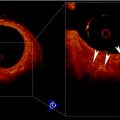 Visualization of Atherosclerotic Coronary Plaque by Using Optical Coherence Tomography
 Segmentation of Carotid Ultrasound Images
 Carotid Plaque Stress Analysis: Issues on Patient-Specific Modeling


Related posts:
Relationship Between Plaque Echogenicity and Atherosclerosis Biomarkers
Quantitative Magnetic Resonance Analysis in the Assessment of Cardiac Diseases
Quantitative Computed Tomography Analysis in the Assessment of Coronary Artery Disease
Visualization of Atherosclerotic Coronary Plaque by Using Optical Coherence Tomography
Segmentation of Carotid Ultrasound Images
Carotid Plaque Stress Analysis: Issues on Patient-Specific Modeling
Stay updated, free articles. Join our Telegram channel
Full access? Get Clinical Tree
