with  the real displacement vector and
  the diffusion time.
In DW-MRI the EAP is estimated by obtaining diffusion-weighted images (DWIs). A DWI is obtained by applying two sensitizing diffusion gradients of pulse length  to the tissue, separated by separation time
  . The resulting signal is ’weighted’ by the average particle movements in the direction of the applied gradient. When these gradients are considered infinitely short (
 ), the relation between the measured signal
  and the EAP
  is given by an inverse Fourier transform (IFT) [2] as
where  is the normalized signal attenuation measured at position
  , and
, and  is the baseline image acquired without diffusion sensitization (
 ). We denote
  ,
,  ,
,  and
and  , where
  and
and  are 3D unit vectors and q,
  . The wave vector
  on the right side of Eq. (1) is related to pulse length
  , nuclear gyromagnetic ratio
  and the applied diffusion gradient vector
  . Furthermore, the clinically used b-value is related to q as
  . In accordance with the Fourier theory, measuring
  at higher
  makes one sensitive to more precise details in
  , while measuring at longer
  makes the recovered EAP more specific to the white matter structure.
to the tissue, separated by separation time . The resulting signal is ’weighted’ by the average particle movements in the direction of the applied gradient. When these gradients are considered infinitely short (), the relation between the measured signal and the EAP is given by an inverse Fourier transform (IFT) [2] as(1)
is the normalized signal attenuation measured at position , and is the baseline image acquired without diffusion sensitization (). We denote , , and , where and are 3D unit vectors and q, . The wave vector on the right side of Eq. (1) is related to pulse length , nuclear gyromagnetic ratio and the applied diffusion gradient vector . Furthermore, the clinically used b-value is related to q as . In accordance with the Fourier theory, measuring at higher makes one sensitive to more precise details in , while measuring at longer makes the recovered EAP more specific to the white matter structure.The relation between the EAP and white matter tissue is often modeled by representing different compartments as pores [10]. Examples of these are parallel cylinders for aligned axon bundles and spherical pores for cell bodies and astrocytes. Several techniques exist to infer the properties of these pores such as their orientation or radius. Of these techniques many sample the 3D diffusion signal exclusively in q-space with one preset diffusion time [3–5]. Among the most used methods is diffusion tensor imaging (DTI) [3]. However, DTI is limited by its assumption that the signal decay is purely Gaussian over  and purely exponential over
  . These assumptions cannot account for in-vivo observed phenomena such as restriction, heterogeneity or anomalous diffusion. Approaches that overcome the Gaussian decay assumption over
  include the use of functional bases to represent the 3D EAP [4, 5]. These bases reconstruct the radial and angular properties of the EAP by fitting the signal to a linear combination of orthogonal basis functions
  with
with  the fitted coefficients. In the case of [5], these basis functions are eigenfunctions of the Fourier transform, allowing for the directly reconstruction of the EAP as
  , where
  . However, these approaches are not designed to include multiple diffusion times, and therefore cannot accurately model the complete 3D+t signal.
and purely exponential over . These assumptions cannot account for in-vivo observed phenomena such as restriction, heterogeneity or anomalous diffusion. Approaches that overcome the Gaussian decay assumption over include the use of functional bases to represent the 3D EAP [4, 5]. These bases reconstruct the radial and angular properties of the EAP by fitting the signal to a linear combination of orthogonal basis functions with the fitted coefficients. In the case of [5], these basis functions are eigenfunctions of the Fourier transform, allowing for the directly reconstruction of the EAP as , where . However, these approaches are not designed to include multiple diffusion times, and therefore cannot accurately model the complete 3D+t signal.The 3D EAP can be related to the mean pore (axon) sizes, e.g. mean volume, diameter and cross-sectional area, by assuming the q-space signal was acquired at a long diffusion time. In this case the diffusing particles have fully explored the tissue structure and thus the shape of the EAP is indicative of the shape of the tissue. This concept was proven in 1D-NMR [7–9] and extended to 3D with the 3D Simple Harmonic Oscillator Reconstruction and Estimation (3D-SHORE) and Mean Apparent Propagator (MAP)-MRI [5] basis. However, this long diffusion time requirement is hard to fulfill in practice as the scanner noise begins to dominate the signal at higher diffusion times.
In contrast, in 1D+t space, Axcaliber [1] samples both over q and  to estimate axon radius distribution. This allows it to overcome the long diffusion time constraint. However, though a 3D-Axcaliber was briefly proposed [6], it is essentially a 1D technique that needs to fit a parametric model to a signal that is sampled exactly perpendicular to the axon direction. While this limits its applicability in clinical settings, this method thickly underlines the importance of including
  in the estimation of axon diameter properties.
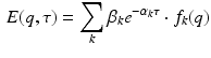
to estimate axon radius distribution. This allows it to overcome the long diffusion time constraint. However, though a 3D-Axcaliber was briefly proposed [6], it is essentially a 1D technique that needs to fit a parametric model to a signal that is sampled exactly perpendicular to the axon direction. While this limits its applicability in clinical settings, this method thickly underlines the importance of including in the estimation of axon diameter properties.Our main contribution in this paper is the generalization of the 3D-SHORE model to include diffusion times. Our new model allows us to obtain analytic representations of the complete 3D+t diffusion space from sparse samples of the diffusion signal attenuation  . In other words, our representation simultaneously represents the 3D+t signal and EAP for any interpolated diffusion time. This allows the time-dependent computation of the orientation distribution function (ODF) previously proposed scalar measures such as the return-to- origin probability (RTOP) and return-to-axis probability (RTAP) [5].
. In other words, our representation simultaneously represents the 3D+t signal and EAP for any interpolated diffusion time. This allows the time-dependent computation of the orientation distribution function (ODF) previously proposed scalar measures such as the return-to- origin probability (RTOP) and return-to-axis probability (RTAP) [5].While our new 3D+t framework opens the door to many new ideas, in this work we consider an initial application of this framework by implementing the Axcaliber model to be used in 3D. In our procedure we first fit our model to a sparsely sampled synthetic 3D+t data set consisting of cylinders with Gamma distributed radii. We then sample an Axcaliber data set from the 3D+t representation perpendicular to the cylinder direction and fit Axcaliber to the resampled data. We compare this method with a previously proposed version of 3D-Axcaliber [6] that uses the composite and hindered restricted model of diffusion (CHARMED) model to interpolate the data points in 3D+t space.
All contributions from this paper are publicly available on the Diffusion Imaging in Python (DiPy) toolkit [19]. http://nipy.org/dipy/.
2 Theory
We propose an appropriate basis with respect to the dMRI signal by studying its theoretical shape over diffusion time  . The effect of diffusion time on the dMRI signal for different pore shapes has been extensively studies by Callaghan et al. [10]. In general, the equations for restricted signals in planar, cylindrical and spherical compartments can be formulated as:
where  and
and  depend on the order of the expansion. Here
  is a function that depends on the expansion order and value of q. The exact formulations can be found in Eqs. (9), (13) and (17) in [10]. As Eq. (2) shows, every expansion order is given as a product of two functions: A negative exponential on
  with some order dependent scaling and a function
  depending only on q. Therefore, an appropriate basis to fit the signal described in Eq. (2) should be a similar product of an exponential basis over
  and another spatial basis over
  . We provide the formulation of our basis in the next section.
. The effect of diffusion time on the dMRI signal for different pore shapes has been extensively studies by Callaghan et al. [10]. In general, the equations for restricted signals in planar, cylindrical and spherical compartments can be formulated as:(2)
and depend on the order of the expansion. Here is a function that depends on the expansion order and value of q. The exact formulations can be found in Eqs. (9), (13) and (17) in [10]. As Eq. (2) shows, every expansion order is given as a product of two functions: A negative exponential on with some order dependent scaling and a function depending only on q. Therefore, an appropriate basis to fit the signal described in Eq. (2) should be a similar product of an exponential basis over and another spatial basis over . We provide the formulation of our basis in the next section.2.1 Specific Formulation of the 3D+t Basis
In accordance with the theoretical model presented in Sect. 2 we fit the 3D+t space with a functional basis that is both separable and orthogonal over both  and
and  . For the temporal aspect of the signal we choose to use an exponential modulated by a Laguerre polynomial, which together form an orthogonal basis over
  . Then, following the separability of the signal, we are free to choose any previously proposed spatial basis to complete our 3D+t functional basis. We choose to use the well-known 3D-SHORE basis [5] as it robustly recovers both the radial and angular features from sparse measurements [11]. Our combined basis finally describes the 3D+t diffusion signal as
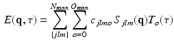
where  is our temporal basis with basis order o and
  is the 3D-SHORE basis with basis orders jlm. Here
  and
and  are the maximum spatial and temporal order of the bases, which can be chosen independently. We formulate the bases themselves as
where  and
and  are the spatial and temporal scaling factors. Here
  ,
,  is a generalized Laguerre polynomial and
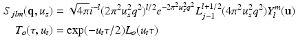
  is the real spherical harmonics basis [12]. Here j, l and m are the radial order, angular order and angular moment of the 3D-SHORE basis which are related as
  with
with 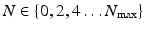 [5].
[5].
and . For the temporal aspect of the signal we choose to use an exponential modulated by a Laguerre polynomial, which together form an orthogonal basis over . Then, following the separability of the signal, we are free to choose any previously proposed spatial basis to complete our 3D+t functional basis. We choose to use the well-known 3D-SHORE basis [5] as it robustly recovers both the radial and angular features from sparse measurements [11]. Our combined basis finally describes the 3D+t diffusion signal as(3)
is our temporal basis with basis order o and is the 3D-SHORE basis with basis orders jlm. Here and are the maximum spatial and temporal order of the bases, which can be chosen independently. We formulate the bases themselves as(4)
and are the spatial and temporal scaling factors. Here , is a generalized Laguerre polynomial and is the real spherical harmonics basis [12]. Here j, l and m are the radial order, angular order and angular moment of the 3D-SHORE basis which are related as with [5].Furthermore, we require data-dependent scaling factors  and
and  to efficiently fit the data. We calculate
  by fitting a tensor
  to the signal values
  for all measured
  . Similarly, we compute
  by fitting an exponential
  to
to  for all measured
  . Lastly, for a symmetric propagator in our 3D+t basis (as is the case in dMRI) we give the total number of estimated coefficients
  as
as

For notation convenience, we use a linearized indexing of the basis functions in the rest of the paper. We denote 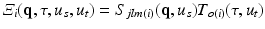 with
with 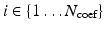 .
.
and to efficiently fit the data. We calculate by fitting a tensor to the signal values for all measured . Similarly, we compute by fitting an exponential to for all measured . Lastly, for a symmetric propagator in our 3D+t basis (as is the case in dMRI) we give the total number of estimated coefficients as(5)
with .Related posts:
 Stable Overlapping Replicator Dynamics for Multimodal Brain Subnetwork Identification
 PET Reconstruction with Sparse Image Representation and Anatomical Priors
Stay updated, free articles. Join our Telegram channel

Full access? Get Clinical Tree


