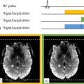
Sylvain MIRAUX1, Frank KOBER2 and Emmanuel Luc BARBIER3,4 1 CRMSB, CNRS, Université de Bordeaux, France 2 CRMBM, CNRS, Université Aix-Marseille, France 3 GIN, Inserm, Université Grenoble Alpes, France 4 IRMaGe, CNRS, Inserm, CHUGA, Université Grenoble Alpes, France Tissue vascularization presents itself as a branched network starting from large vessels (~1 cm in diameter in humans) and finishing with capillaries (~6 µm in diameter). Capillaries are where the exchanges between blood and tissues occur. Two main types of vascular imaging exist: flow and perfusion imaging. This is not a biological distinction; it is related to spatial resolution. For example, let us consider a 1 mm pixel: In vascular imaging, it is common to use contrast agents, similar to the colorants used to track water in rivers. The properties of contrast agents are detailed in section 6.2. In order to understand their use, let us recall a few basic physiological notions. Blood contains cells and plasma. The percentage of red cells is called the hematocrit. It is approximately 15% lower in capillaries than in large vessels. Blood cells and plasma do not circulate at the same speed. In other words, blood is not a homogeneous liquid, and contrast agents circulate like plasma. Blood circulation can be represented as vascular loops that start from the heart and return to the heart: for example, the heart–brain, right arm–heart or heart–heart loops. At the end of each loop, there is a capillary network. Blood flow is not uniform along the loop. For instance, it varies from about 50 cm/s in the aorta (in reality a very variable speed, due to the cardiac pulsations) to 0.1 cm/s in the capillaries, and up to 30 cm/s on average in the veins that reach the heart. Venous blood arriving at the heart is then directed toward the lungs, where it becomes oxygenated, returns to the heart and leaves it again via the aorta, the largest arterial trunk in the body. Contrast agents must modify the MRI signal but not the physiology. Therefore they consist of chemically and biologically inert molecules that do not modify the blood behavior (so-called tracers). A very low volume (about 10–20 mL of solution), compared to the blood volume, is typically injected into an arm vein. To allow the contrast agent to reach the organs in the most compact way and in the shortest time (a bolus), a physiological serum is injected after the contrast agent to quickly push the latter from the arm vein to the vena cava. After the small circulation (heart–lung–heart), it is ejected into the aorta at physiological pressure. A first pass of contrast agent occurs in each organ. Due to the branching of the vascular network at the end of each loop, the contrast agent becomes more diluted when flowing through an organ. Furthermore, the contrast agent gradually leaves the vascular bed: it is extracted at the kidneys and liver and, if its hydrodynamic diameter is sufficiently small (the molecule’s diameter, including its hydration layer) and if the vessel walls are permeable, it also spreads in tissues. After some minutes, the contrast agent concentration in the blood gradually decreases, typically over several hours. This slow decrease is characterized by the plasmatic half-life of the contrast agent. It should be noted that the vast majority of vessels are permeable to contrast agents, except in a healthy brain where the vessel walls constitute a barrier, called the blood–brain barrier (BBB). Since MRI detects protons of water, several preclinical experiments have investigated the delivery of contrast agents using other nuclei, such as fluorine. In practice, chemistry and the need for specific equipment are not favorable for their routine usage in clinics. Therefore, clinical settings employ agents that influence the water signal. The matter’s behavior inside a magnetic field is characterized by magnetic susceptibility, denoted as ?. Water and biological tissues are usually diamagnetic: when they are placed into a magnetic field, they produce very weak magnetization that opposes the magnetic field. Their magnetic susceptibility is negative and very low (water: –9.05 × 10⁻⁶; human tissues: between –11 × 10-6 and –7 × 10⁻⁶) (Schenck 1996). Conversely, contrast agents are paramagnetic or superparamagnetic: when placed inside a magnetic field, they produce a magnetization oriented along the magnetic field. Their magnetic susceptibility is positive, with the susceptibility of superparamagnetic agents greater than that of paramagnetic agents. All contrast agents produce two types of effects on the MRI signal, a relaxivity effect and a susceptibility one. Paramagnetic or superparamagnetic contrast agents accelerate the spin-spin (T2) and spin-lattice (T1) relaxation processes. At a molecular level, thermal oscillations of the contrast agent produce small and rapid local fluctuations of the magnetic field. The frequency component that corresponds to the magnetic resonance of water molecules accelerates the relaxation of water located in the hydration layer of the contrast agent. For a given condition of the magnetic field, temperature and biological environment, the relaxation power or relaxivity of a contrast agent is characterized by two values: r1 and r2. For a homogenous liquid, this can be written as: where T1AC (respectively, T2AC) is the T1 (respectively, T2) in the presence of a contrast agent, T10 (respectively, T20) is the T1 (respectively, T2) in the absence of a contrast agent, r1 (respectively, r2) is the relaxivity (mMol-1·s-1) and [AC] is the contrast agent concentration in mMol. Some generic observations on the relaxivity effects should be highlighted: if the membranes hinder the water molecules’ motion, the relaxivity effect is reduced. The greater the magnetic field intensity, the lower the relaxivity effect. The larger the hydrodynamic diameter of the contrast agent, the stronger the relaxivity effect. Moreover, T1 and T2 effects are opposite: when T1 decreases, the signal level usually increases; when T2 decreases, the opposite occurs. Thus, for a spin echo sequence, the relationship between the signal and the contrast agent concentration follows a bell-shaped curve: at low concentrations, the T1 effect is dominant and the signal amplitude increases with the concentration. At higher concentrations, the T2 effect becomes dominant and the signal amplitude decreases with the concentration. The bell-shaped curve of signal level as a function of concentration is not bijective and leads to quantification difficulties. The magnetic susceptibility effect is based on the perturbation of the magnetic field lines in the vicinity of the contrast agent. Since the magnetic field around the contrast agent is non-uniform, the spins of hydrogen atoms situated nearby gradually dephase and the magnitude of the vector sum of these spins – the magnetization – becomes lower than in the absence of a contrast agent. This effect, related to T2* (non-uniformity of the magnetic field at a microscopic level), is distinctly visible in gradient echo images and less visible with spin echo sequences. Some generic observations on the susceptibility effect can be made: the membranes have no impact on this effect. Moreover, the stronger the magnetic field, the greater the susceptibility effect. Finally, the larger the contrast agent’s diameter, the greater the susceptibility effect (one may consider that the effect extends over a distance equivalent to the diameter of the contrast agent). Therefore, contrast agent molecules that are gathered in the same biological compartment (capillary, cell, vesicle) will have a greater susceptibility effect than if they were relatively uniformly distributed in the same volume of tissue. The inverse phenomenon occurs for the relaxivity effect: it will be maximum if the contrast agent is uniformly distributed in the biological tissue. Superparamagnetic contrast agents have a larger diameter and lead to greater susceptibility effects than paramagnetic contrast agents. However, today, their clinical use in humans is not approved, because their benefit compared to existing contrast agents has not been demonstrated. Numerous MRI sequences exist for visualizing large vessels (veins and arteries). Typically, they are adapted to the type of investigated vessels and their location and can be divided into three large categories: Figure 6.1. Gradient waveforms (1; (– 1)) and (1; (– 2); 1) and plots showing the accumulated phase as a function of time for stationary spins and spins with a constant velocity We shall describe the physical principle of each method with their advantages and disadvantages and show images of examples. Finally, we shall mention the most recent time-resolved techniques that not only detect the location of the blood vessels but also visualize the blood motion in these vessels. As a foreword, we shall tackle the principle of gradients and flow compensation (Simonetti et al. 1991; Parker et al. 2003). This gradient pattern is almost always employed in angiography sequences (TOF, phase and sometimes even with T1 contrast agents) and dynamic angiography. Figure 6.1 illustrates the principle of flow compensation via gradients. In a standard gradient echo sequence (1;(– 1) pattern), only the stationary spins are rephased at the end of the gradient pattern. Conversely, moving spins are dephased, which consequently causes a decrease or even absence of their signal. To address this problem, patterns such as 1;(– 2);1 can be used to rephase moving spins. All of this can only be done at the price of a longer TE in the sequence. A 1;(– 2);5;(– 2);1 pattern can be also used to compensate for the dephasing of spins with a constant acceleration. White-blood and “time-of-flight” (Laub 1995) imaging sequences are basic slice-selective gradient echo sequences. However, they include the feature of flow compensation. Today, these sequences are mostly used in three dimensions for angiography applications. For this reason, they employ very short repetition times TR (<25 ms) compared to the longitudinal spin relaxation time T1 in order to keep the acquisition time of a volume short. Most of all, however, the usage of short TR causes the attenuation of the signal from stationary spins due to the “saturation” or “partial saturation” effect. This effect becomes more pronounced as the TR/T1 ratio decreases. In the case of a 3D volume with slice selection, stationary spins (i.e. spins in muscle tissues and gray and white matter) are directly affected by this phenomenon and exhibit a strongly attenuated signal. Conversely, blood spins, that is, moving spins, exhibit no or only partial effect of the saturation phenomenon as they are not always present in the imaging slice during the entire scan. This mechanism is described with the name “flow-related enhancement” or “entry slice phenomenon”. It increases with flow velocity, the vessel’s orthogonal orientation with respect to the slice, and decreases with slice thickness (Figure 6.2). In practice, TOF angiography imaging is performed for vessels in the brain (visualization of the Willis polygon) and in the neck (carotid arteries). In the brain, the MOTSA (multiple overlapping thin slab acquisition) (Davis et al. 1994) or sequential 3D TOF technique is used. By acquiring three or four small volumes, it maximizes the flow-related enhancement effect while reducing the scan time. The sequence is flow-compensated and employs the parameters described below (at 3 T). This type of sequence becomes more efficient at higher magnetic fields. As stationary spins’ T1 is longer at 3 T than at 1.5 T, these spins are more saturated. The TOF phenomenon, on the other hand, is less sensitive to the magnetic field intensity. Figure 6.2. Schematic of the “time-of-flight” principle. The images are extracted from a 3D volume with a selection of slices of 2 cm and 4 cm thickness. The “time-of-flight” effect highlights vessels with a strong signal (red arrows). It is more prominent when the slice thickness is smaller. Some vessels visible on the 2 cm slice are not visible any longer on the 4 cm slice (dashed arrows) To increase the quality of TOF images, in particular in terms of contrast, several blocks can be used at the beginning of the sequence (magnetization transfer, fat suppression; Atkinson et al. 1994). To reduce the saturation phenomenon at the end of the slice, radiofrequency pulses with variable flip angles can be employed (TONE; Saib et al. 2019). ACQUISITION PARAMETERS FOR A TOF SEQUENCE AT 3 T.– FLASH 3D sequence with four adjacent selective slices of 2 cm: TE/TR = 3.42/21 ms; flip angle: 18°; field of view: 200 × 181 mm; resolution: 0.3 × 0.3 × 0.5 mm; phase acceleration factor: 2; in-slice partial Fourier: 7/8; acquisition time: 5:33 min. The goal of contrast agents used in angiography is to modify the relaxation times of the blood (Prince 1994). The most employed contrast agent is gadolinium in a chelated form (Weinmann et al. 1984). An injector is used to accurately control the dose and speed during the injection. Similar to TOF imaging, 3D gradient echo sequences are used. Contrary to the former method, no specific slice positioning is necessary. Indeed, the signal enhancement is uniform within the vessels. However, the acquisition speed is the most important criterion to be taken into account. Sequences with large receive bandwidths, short TR (<10 ms), partial Fourier acquisition and parallel imaging techniques are employed. One of the challenges of this type of method is the synchronization of the acquisition with the first pass of a contrast agent inside the arterial system. Often, a 2D sequence combined with a pre-bolus with a small volume is used to determine the optimum timing of the 3D acquisition. In these approaches, the center of the k-space must be acquired at the moment of the contrast agent’s first pass in the arterial system such that the acquisition is not “contaminated” by the signal from the venous system. Elliptical acquisitions that start from the k-space center are used (Wilman et al. 1998). Advancements in the domain of parallel imaging enable dynamic image acquisitions with a coarser spatial resolution that show and confirm the first pass. By combining these techniques with advanced reconstruction methods, it is possible to reconstruct high-resolution images of the first pass a posteriori. The venous system visualization, in contrast, presents fewer constraints in terms of acquisition time and high-resolution images can be acquired in this case (Farb et al. 2003). ACQUISITION PARAMETERS WITH CONTRAST AGENT.– 3D FLASH sequence: TE/TR = 1.2/4.4 ms; flip angle: 20°; field of view: 160 × 160 mm; resolution: 0.5 × 0.5 × 0.5 mm; phase acceleration factor: 2; in-slice partial Fourier: 7/8; elliptical centric phase-encoding; acquisition time: 54.8 s. The main difficulty in white-blood imaging is the lack of a positive signal. Its main possible cause is a too-slow blood velocity in the vessels in TOF imaging. In particular, this occurs in pathologies such as aneurysms, where the blood’s circulation velocity is decreased. In these conditions, a contrast agent is added to compensate for the reduced signal. Intra-voxel dephasing is also a cause of low blood signal in TOF imaging due to turbulent flows with variable velocity. In contrast-agent imaging, the main cause of the lack of signal lies in a poor synchronization of the bolus injection with the readout of the k-space center. The T2* effect caused by adding contrast agents at high concentrations can also lead to signal loss, which can be compensated by reducing the TE of the sequence. Phase contrast imaging was introduced in 1982 by Moran (1982) and its 3D version by Dumoulin et al. (1989). The goal of this method is to acquire images of spin circulation by applying flow-encoding gradients. In phase imaging, velocity encoding gradients translate flow velocity into phase values. In practice, a bipolar gradient is applied during a gradient echo sequence. The gradient applies a phase to the magnetization that is linearly proportional to the velocity. This gradient is called the “velocity encoding gradient”. The axis along which the gradient is applied determines the direction of flow sensitivity. Such gradients can be added to a gradient echo sequence along three spatial directions. In practical implementations, two sets of images are acquired with the same parameters, except for the first moment of the bipolar gradients. The two images are then subtracted pixel by pixel. This method provides images where the pixel’s intensity is directly related to the flow velocity. Generally, flow is displayed with a positive sign when it has the same direction as the bipolar gradient and a negative sign when it has the opposite orientation. Stationary spins have an average signal (gray) with a zero phase. To obtain a flow image without direction information, the absolute value is obtained from the combination of the phase images of the three orthogonal flow-encoding directions; this represents a “velocity” image. The amount of velocity encoding is defined by the variation in the moment between two bipolar gradients. To quantify this, the VENC (Velocity ENCoding, expressed in cm/s) parameter is introduced in phase imaging, and its value is determined before the scan by the operator. This value is positive and inversely proportional to the difference of the first gradient moments according to the following equation: where ∆m1 is the variation of the first moment of the bipolar velocity gradient (when the gradient waveform is executed). Contrary to TOF and contrast agent methods, the phase contrast imaging technique is not often used. The reason lies in the relatively long acquisition time for this method due to the need to combine several images. However, this approach is compatible with parallel acquisition techniques, and its acquisition time can be significantly reduced in such a way. The phase contrast technique is mainly used for intracranial angiography. However, although it was initially developed for acquiring images of blood vessels, phase-based techniques are widely employed in other applications (measurements of motion, temperature imaging, CSF flow imaging, etc.). SEQUENCE ACQUISITION PARAMETERS.– Phase contrast 3D sequence (EG) with VENC 40 cm/s and four slices of 2 cm: TE/TR = 6.49/44.2 ms; flip angle: 10°; field of view: 240 × 180 mm; resolution: 0.5 × 0.5 × 0.9 mm; phase acceleration factor: 2; in-slice partial Fourier: 7/8; acquisition time: 3:59 min. Black- (or dark-)blood imaging is another type of angiography technique. As indicated by the name, the principle underlying these methods is to suppress the blood signal and thereby visualize its location with respect to stationary tissues by observing a negative effect in blood vessels. Such methods must strongly attenuate the blood signal while preserving the signal from surrounding stationary tissues. Diminishing or suppressing the blood signal is achieved via sequences exploiting the “exit slice” effect. This phenomenon is found in most standard spin echo methods, whether accelerated (RARE) or not (conventional spin echo). As illustrated in Figure 6.3, while stationary spins are subjected to the effect of a 90° pulse followed by a refocusing 180° pulse to generate a spin echo, moving spins are subjected to only one of the two pulses. Therefore, their signal is almost non-existent in the images. This effect becomes more prominent as the spin velocity increases. In practice, a saturation slice can be used before the image acquisition to suppress the signal from slowly moving spins in an even more efficient way. Other sequences can be employed to suppress the blood signal, such as inversion recovery (Mayo et al. 1989) or double inversion recovery (Simonetti et al. 1996) sequences. Figure 6.3A. Principle of black-blood imaging using a spin echo sequence Figure 6.3B. Images obtained in the same volunteer with white-blood and black-blood methods to visualize the carotid arteries (pink arrow) Black-blood sequences are typically used for imaging of the heart or vessel walls (e.g. in carotid vessels) to better detect stenosis or atheromatous plaques. In the case of cardiac imaging, the sequences are synchronized with the electrocardiogram (ECG) signal. In such conditions, the sequence has to be perfectly synchronized to acquire the images during the most static phase of the heart while efficiently suppressing the blood signal. Acquisition parameters for a T2 black-blood sequence at 3 T are the following: 2D spin echo sequence; TE/TR = 123/1,300 ms; flip angle: 10°; field of view: 220 × 171 mm; voxel size: 0.9 × 0.9 × 0.9 mm; phase acceleration factor: 2; in-slice partial Fourier: 6/8; enabled fat suppression; acquisition time: 5:17 min. An alternative to black-blood sequences consists of using the T2* of the deoxyhemoglobin in the blood. Such an approach is called SWI imaging, or susceptibility-weighted imaging, and it produces a black blood venogram. In practice, a 3D volume is acquired with a gradient echo sequence with a long TE (> 15 ms at 3 T). Magnitude and phase images are reconstructed from the same raw k-space data. Phase images are filtered with a high-pass filter to remove any phase that is not due to local susceptibility variations. Since phase images are more sensitive to variations than magnitude images, they are used to calculate an image mask which is multiplied by the magnitude image (Haacke et al. 2004). Figure 6.4 (right) shows an SWI image of a volunteer’s brain. In black-blood imaging, contrary to TOF imaging, turbulent flows represent an advantage. This is especially the case in areas with a complex flow such as stenoses, where TOF imaging can prove inefficient, while black-blood angiography can enable pathology detection with better specificity. The main inconvenience of black-blood sequences is their low SNR, as well as the difficulty in applying them in three dimensions for high-resolution imaging. SWI imaging, on the other hand, is by definition very sensitive to susceptibility effects, which can lead to a lot of artifacts that make image interpretation impossible. Several other angiographic techniques have been developed that are neither white-blood, black-blood nor contrast agent techniques. This research area is very active, as MRI is a very good alternative to Angio-X methods thanks to its harmlessness. Among these techniques, fresh blood imaging (Miyazaki et al. 2000) provides images of the extremities with very good contrast. Balanced SSFP (Fan et al. 2009) or quiescent-interval single-shot (QISS) (Edelman et al. 2010) sequences are also employed for lower limb imaging. Finally, spin marking approaches can prove as efficient as invasive catheter-based methods (Grist et al. 2012). Figure 6.4. Brain angiography of the same volunteer with a 3D TOF, 3D phase contrast and SWI sequence. The visualization is done using maximum intensity projection (MIP) and minimum Intensity Projection (mIP) algorithms for white-blood and black-blood imaging, respectively Today, thanks to advances in hardware, in particular with parallel imaging, it is possible to acquire time-resolved angiographic images, whether with or without contrast agents and even with phase imaging (Markl et al. 2012). These methods are typically based on the utilization of acceleration techniques such as keyhole, compressed sensing or alternative methods such as VIPR (radial 3D Vastly undersampled Isotropic PRojection) (Mistretta 2009). These methods acquire less spatially resolved images than anatomical angiographic techniques. Nevertheless, the obtained information makes them an alternative to invasive fluoroscopy methods. Becoming established in the clinical routine is a long and tedious process. This is due to the long acquisition time and the complex processing techniques that need to be implemented. As described by the method’s name, the dynamic susceptibility contrast (DSC) approach is based on the susceptibility effect of a paramagnetic contrast agent. This is injected in the form of a bolus and MRI acquisition is done dynamically to capture the first pass of the contrast agent in the blood circulation. This approach is particularly suitable for the brain: due to the BBB, the contrast agent remains confined to the vessels. In this context, the central volume principle, a mathematical model, relates the measurement of the contrast agent’s concentration evolution to the estimation of physiological parameters that characterize perfusion. In DSC, T2* weighted sequences are typically used since they are sensitive to susceptibility effects. To obtain a temporal resolution of about 1.5 s and good spatial coverage, gradient echo EPI sequence is mainly utilized. It is recommended that approximately 30 s of signal is acquired to obtain a robust estimation of the baseline signal (the signal before the appearance of the contrast agent). The entire scan typically lasts between 1 and 2 minutes. Its goal is to properly sample the first pass of the contrast agent and, if possible, some time afterward. In the case of vascular anomalies (e.g. cerebral stroke), a 2 min acquisition is recommended. Due to the spatial coverage and time resolution constraints, spatial resolution is typically between 2 and 4 mm. Initially obtained with segmented acquisitions and thus shorter TR than the temporal resolution indicated above, these acquisitions used to be sensitive to T1 variations (relaxivity effects). Today, parallel imaging approaches (e.g. SENSE) enable non-segmented acquisitions and thus reduce these T1 effects by employing long TR. Multi-band acquisitions (simultaneous excitation of several slices) offer new perspectives to make the scans even more robust to T1 effects via the acquisition of several echoes for measuring the T2* effect and compensating for it during the analysis. Finally, some groups use spin echo EPI sequences, hence T2 weighted, to achieve higher sensitivity to small vessels, although the signal-to-noise ratio is lower than in gradient echo sequences. We shall come back to this aspect in section 6.4.3. In the 1990s, numerical simulations and mathematical models explored the relationship between MRI signal variations and the changes in contrast agent concentration. These approaches were based on strong hypotheses, such as a uniform distribution of the vessels’ directions (i.e. without a preferential orientation), a unique vessel diameter, absence of interactions between the contributions from the different vessels, small blood volume and a constant difference in magnetic susceptibility between intra- and extra-vascular compartments (this difference is caused by the contrast agent concentration and the employed magnetic field). In 1994, Yablonskiy and Haacke (1994) published a set of equations that demonstrated a linear relationship between the volume occupied by the vessels and the variation of the gradient echo signal due to the magnetic susceptibility effect. In 1995, Boxerman et al. (1995) published numerical simulations investigating the MRI signal change induced by a given contrast agent concentration. They have studied the signal variation for gradient echo sequences – characterized by ∆R2*, that is, the difference between R2*=1/T2* with and without contrast agent – and spin echo sequences. If the above-mentioned hypotheses are true, ∆R2* is proportional to the contrast agent concentration. Several elements should be highlighted here: Two main approaches are used for signal analysis: the oldest consists of an analysis of the curve features and its most recommended version employs the arterial input function (AIF) to obtain data that is well-quantified as possible via a sensitive deconvolution step (Willats and Calamante 2013). Actually, up to the current day, it is not possible to extract absolute quantitative maps of blood flow or volume. Due to this fact, there is no clear consensus on the best analysis method. In the classic approach, the following formula is calculated:
6
Vascular Imaging: Flow and Perfusion
6.1. Introduction
6.2. Contrast agents
6.2.1. Biological behavior
6.2.2. Diamagnetism, paramagnetism and superparamagnetism
6.2.3. Relaxivity effect

6.2.4. Susceptibility effect
6.3. Angiography

6.3.1. White-blood imaging
6.3.1.1. “Time-of-flight” imaging

6.3.1.2. Contrast agent imaging
6.3.1.3. White-blood imaging limitations
6.3.2. Phase contrast imaging

6.3.2.1. Limitations of phase contrast imaging
6.3.2.2. Usage
6.3.3. Black-blood imaging


6.3.4. Other techniques

6.3.5. Dynamic angiography
6.4. Perfusion imaging
6.4.1. Dynamic susceptibility contrast

Related posts:
Stay updated, free articles. Join our Telegram channel

Full access? Get Clinical Tree


