Vascular Ultrasound
William E. Brant
Raymond S. Dougherty
Spectral Doppler US and color-flow vascular imaging supplement gray-scale US by identifying blood vessels, confirming the presence of blood flow determining flow direction, detecting vessel stenosis and occlusion, assessing the perfusion of organs and tumors, and characterizing blood flow dynamics to detect physiological abnormalities. This chapter reviews the basics of vascular US examination and Doppler interpretation (1,2,3,4).
Doppler Basics
Doppler effect refers to the change in the frequency of sound waves that occurs due to motion of a sound source, a sound reflector, or a sound receiver. Johann Doppler of Salzburg Austria described this phenomenon in 1842. In medical diagnosis, the Doppler effect is used to confirm blood flow by detecting the change in frequency of US waves that occurs when sound is reflected from moving clumps of red blood cells (RBCs). The echoes reflected from RBCs are very weak, having a signal intensity up to 10,000 times less than that of contiguous soft tissue; thus, Doppler US instruments require a high sensitivity to weak signals, and instrument settings must be routinely optimized.
Doppler shift is the change in frequency between the US waves emitted by the transducer and the US waves returning to the transducer after reflection from moving RBCs (Fig. 39.1). This shift in sound frequency results from the Doppler effect. The reflected sound frequency increases when the blood flow direction is toward the Doppler signal and decreases when the direction is away from the Doppler signal. An increase in frequency is termed a positive Doppler shift; the sound waves are compressed by encountering RBCs moving toward the sound source. A decrease in frequency is termed a negative Doppler shift as the reflected sound waves are stretched by RBCs moving away from the sound source. The presence of a Doppler shift within a blood vessel confirms the presence of blood flow. The direction of the Doppler shift toward higher or lower frequency indicates the direction of blood flow. Doppler shift frequencies are within the range of human hearing and produce distinctive audible sound patterns that characterize normal and abnormal arterial and venous blood flow.
Doppler Equation. The Doppler equation describes, in mathematical form, the relationship between the Doppler frequency shift (ΔF) and the velocity (V) of the moving RBCs that produce the shift.
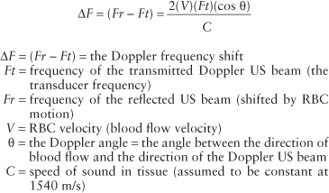
The frequency shift (ΔF) is proportional to the following: (1) the velocity (V) of the moving RBCs; (2) the frequency of the transmitted Doppler US beam (Ft); and (3) the cosine of the angle between the incident Doppler US beam and the direction of blood flow. This angle is called the Doppler angle and is symbolized by the Greek letter theta (θ). The direction of blood flow is assumed to be parallel to the walls of the visualized blood vessel being interrogated (Fig. 39.2). The Doppler US beam can be steered by controls on the US unit. The direction of the Doppler beam is indicated on the US image by a dotted or dashed line.
The fact that the Doppler frequency shift is directly proportional to the cosine of the Doppler angle has important implications (Table 39.1). First, the largest frequency shift—that is, the largest Doppler signal—will be obtained when the Doppler US beam is directed straight down the barrel of the vessel (θ = 0°, cosine 0° = 1). Second, no Doppler shift will occur when the Doppler US beam is directly perpendicular to blood flow (θ = 90°, cosine 90° = 0). Small errors in Doppler angle estimation cause only small errors in velocity calculations at small Doppler angles, but small errors in Doppler angle estimation cause large errors in velocity calculations at angles close to
90°. As a general rule, Doppler scanning should be performed to keep Doppler angles at 60° or less.
90°. As a general rule, Doppler scanning should be performed to keep Doppler angles at 60° or less.
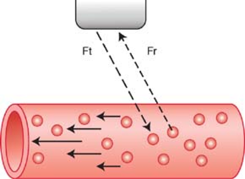 Figure 39.1. Doppler Frequency Shift. The transmitted Doppler US beam (Ft) encounters red blood cells (RBCs) moving toward it within a visualized blood vessel. The RBC motion causes an increase in frequency of the returning echo (Fr) due to the Doppler effect. The US instrument detects and measures the frequency of the returning Doppler signal, confirming the presence of blood flow and its direction by the presence and direction of the Doppler frequency shift. |
By algebraic manipulation, we can rewrite the Doppler equation as follows:
The US unit detects and measures the frequency of the Doppler beam reflected from moving RBCs (Fr) and calculates the Doppler frequency shift (ΔF = Ft – Fr). The transmission frequency (Ft) is determined by the transducer chosen to perform the examination. The speed of sound in human tissue is assumed to be constant (C). The operator communicates the Doppler angle to the US unit by aligning the Doppler angle “wings” to be parallel with the walls of the vessels examined (Figs. 39.2, 39.3).
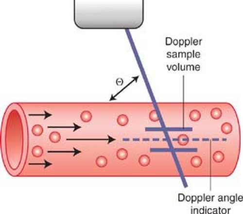 Figure 39.2. Doppler Angle. The Doppler angle, θ, is defined as the angle between the Doppler US beam and the direction of blood flow, which is assumed to be parallel to the walls of the blood vessel. The Doppler sample volume is indicated by two parallel lines. The Doppler angle indicator is displayed as a dashed line within the sample volume. The US unit has a control knob that is used to align the Doppler angle indicator with the blood vessel walls. |
Table 39.1 Cosine Values | ||||||||||||||||||||||
|---|---|---|---|---|---|---|---|---|---|---|---|---|---|---|---|---|---|---|---|---|---|---|
|
Because the depth of a structure in an US image is measured by the time delay between transmission of the US into tissue and the return of the echo from the structure, we can limit Doppler information to a selected Doppler “sample volume” by use of a “time window.” The length of the time window determines the size of the sample volume and the time delay of the time window determines its depth. Thus, we can restrict Doppler information to a small portion of a single visualized vessel. On most Doppler US units, the size and location of the Doppler sample volume is indicated by two short parallel lines along the Doppler beam indicator line (Figs. 39.2, 39.3). Simultaneous gray-scale imaging and Doppler scanning is called duplex US. Both spectral and color Doppler (CD) imaging are examples of duplex imaging.
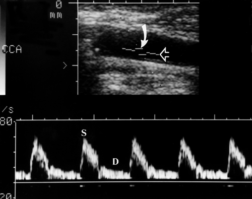 Figure 39.3. Duplex Doppler US. US image shows the Doppler spectrum of the common carotid artery. The vertical scale shows blood flow velocity in meters per second. The horizontal scale shows time in seconds. The Doppler trace demonstrates peak velocities in systole (S) and low flow velocities in diastole (D). A 2-mm Doppler sample volume (curved arrow) is placed by the sonographer in the midportion of the artery visualized by real-time US. Only Doppler shifts originating from this sample volume are analyzed for display. An estimated Doppler angle of 50° is communicated to the US unit computer by aligning the angle indicator (open arrow) parallel to the vessel walls. |
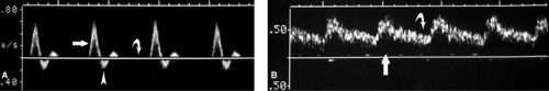 Figure 39.4. High-Resistance and Low-Resistance Doppler Spectrum. A. A high-resistance waveform is characterized by rapid systolic upstroke (straight arrow), low flow velocities, or no flow, during diastole (curved arrow), and, commonly, reversal of flow direction (arrowhead) in early diastole. This Doppler spectrum was obtained from the common femoral artery. B. A low-resistance waveform is characterized by relatively high flow velocities throughout diastole (curved arrow). The narrow spectrum and clean systolic window (straight arrow) is characteristic of laminar blood flow. This Doppler spectrum was obtained from the internal carotid artery. |
Doppler Spectral Display. Returning Doppler signals are processed using a fast Fourier transform spectrum analyzer that sorts the range and mixture of Doppler frequency shifts into individual components and displays them as a function of time on a velocity (or frequency shift) scale (Fig. 39.3). Analysis is performed rapidly enough to be displayed in real time. The horizontal scale (x-axis) of the Doppler spectrum represents time in seconds. The vertical scale (y-axis) represents blood flow velocity in m/s or cm/s. Because velocity and Doppler frequency shift are directly related mathematically, Doppler frequency shift may alternatively be used on the vertical scale without changing the appearance of the Doppler spectrum. Since the blood flow velocity provides the most diagnostically useful information, velocity is the usual choice for the vertical axis. Each pixel (dot) in the spectral display represents a group of RBCs moving at a specific velocity at a given moment in time. The more RBCs moving at that specific velocity and time, the brighter the pixel. Flow toward the Doppler beam (positive frequency shift) is displayed above the zero baseline and flow away from the Doppler beam (negative frequency shift) is displayed below the zero baseline. Peaks of higher velocity occur during ventricular systole and periods of lower velocity represent ventricular diastole.
Spectral Waveforms. Different blood vessels have unique flow characteristics that can be recognized by the Doppler spectral waveform (Doppler “signature”) they produce (5,6,7). Factors that affect the appearance of the spectral waveform include cardiac contraction, vessel compliance, and downstream vascular resistance. Cardiac arrhythmias are reflected in the periodicity of the systolic peaks and the velocities reached during each cardiac contraction. A major determinant of the spectral waveform’s appearance is the resistance to blood flow offered by the vascular bed supplied by the artery being studied. Arteries can be categorized as high resistance or low resistance based upon their Doppler spectral waveform. High-resistance spectral waveforms are characterized by velocities that increase sharply with systole, decrease rapidly with the cessation of ventricular contraction, and show little or no forward flow during diastole (Fig. 39.4A). Blood flow direction may reverse briefly during early diastole producing a triphasic waveform. Blood flow in high-resistance arteries is always under considerable pressure and encounters constricted arterioles that impede forward blood flow. Pulse pressures traveling down the arterial tree are highly reflected, which results in minimal flow to the capillary bed during diastole. Diastolic flow velocity is low, absent, or reversed, and pulse pressure is high. The ratio of systolic velocity to diastolic velocity (pulsatility) is high. Arteries that normally show a high-resistance pattern Doppler waveform include arteries that supply primarily skeletal muscle at rest including the iliac, femoral, popliteal, subclavian, and brachial arteries. The external carotid artery (ECA) waveform is relatively high resistance in appearance. Low-resistance spectral waveforms are characterized by a slower increase in flow velocity with the onset of systole and a gradual decrease in velocity during diastole with continued forward flow throughout the cardiac cycle (Fig. 39.4B). Arteries that supply vital organs characteristically have a low-resistance waveform. These include the internal carotid artery (ICA), hepatic arteries, and the renal arteries. The superior mesenteric artery waveform has a high-resistance pattern during fasting and a low-resistance pattern after eating, thus reflecting opening of intestinal tract arterioles and increased intestinal blood flow induced by food in the gut. The common carotid artery (CCA), with 70% of its blood flow going to the ICA, has a low-resistance spectral waveform.
Laminar Blood Flow. Most normal arteries and large veins have a laminar pattern of blood flow. The blood flow velocity is highest at the center of the vessel and progressively diminishes closer to the vessel wall (Fig. 39.5). The Doppler waveform of laminar flow is characterized by a “narrow spectrum”—a narrow band of blood flow velocities throughout the cardiac cycle with a “window” beneath the spectral trace in systole (Fig. 39.5). Large arteries such as the aorta have “plug” flow characterized by uniform flow velocities extending from the center to near the vessel wall. At vessel bifurcations, the division of blood flow results in a small area of normal reversed blood flow near the vessel wall opposite the flow divider (Fig. 39.6). Tortuous blood vessels demonstrate normal slowing of blood flow on the inner aspect of the curve with acceleration of blood flow on the outer aspect of the curve. The highest velocities are seen at the outer aspect of the curving vessel, rather than at midlumen. Blood flow velocity returns to a laminar distribution a short distance downstream from the curve.
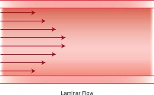 Figure 39.5. Laminar Blood Flow. Blood flow in most normal arteries is arranged in an orderly layering pattern, with the highest velocity in the midstream and the lowest velocity near the vessel wall. |
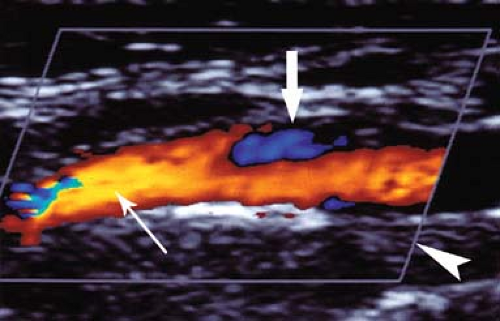 Figure 39.6. Normal Flow Reversal at Bifurcation. Flow in the internal carotid artery is shown in red with areas of higher flow velocity shown in yellow. A normal area of blood flow reversal (fat arrow) is seen in the carotid bulb. Note how the true color change is outlined in black. The color Doppler interrogation area is marked on the image by the box outlined in white (arrowhead). Higher velocity in the middle of the vessel, shown in yellow (thin arrow), is indicative of laminar blood flow in the artery. |
Disturbed Blood Flow. Turbulent and disturbed spectral waveforms are usually, but not always, indicative of pathological changes in blood flow. Disturbed blood flow is a loss of the normal orderly laminar flow pattern. Characteristic spectral Doppler signs of disturbed blood flow are increased velocity, spectral broadening, simultaneous forward and reverse flow, and fluctuations of flow velocity with time (2,4). Peak systolic velocity (PSV) increases with severity of vessel stenosis. Spectral broadening is widening of the spectral waveform that reflects a broader range of flow velocities within the Doppler sample volume. Spectral broadening increases with the severity of flow disturbance. However, normal spectral broadening occurs when the size of the Doppler sample volume is large compared to the size of the vessel, or when the sample volume is placed near the vessel wall instead of midlumen. Flow velocity fluctuation and simultaneous forward and reverse flow characterize turbulence. Turbulence is most pronounced just downstream from a severe vessel stenosis where eddy currents are produced as the high-velocity flow slows and occupies a larger vessel area.
Velocity Ratios. Blood flow velocity calculations are dependent upon accurate estimation of the Doppler angle. When the Doppler angle cannot be determined due to poor visualization of the interrogated blood vessel or the vessel’s tortuosity (as with the umbilical artery in the cord), velocity cannot be accurately calculated. When the Doppler angle indicator is not displayed, the US instrument calculates Doppler velocities using Doppler equation by assuming the Doppler angle is 0° (cosine 0° = 1). Velocity ratios can be calculated from the spectral waveform and can be used to estimate vascular resistance and hemodynamics. The ratios are independent of absolute velocity measurements. The velocity ratios in common use are listed in Table 39.2.
Table 39.2 Doppler Velocity Ratios | |
|---|---|
|
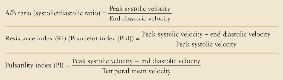
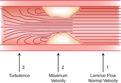 Figure 39.7. Assessing Arterial Stenosis. To assess a vessel plaque for stenosis, Doppler spectra are obtained (1) proximal to the plaque where the blood flow velocity is normal and the flow is laminar; (2) in the area of the plaque where the flow usually remains laminar but where flow velocity is at maximum; and (3) downstream from the plaque where turbulence and eddy currents are detected. |
Assessing Arterial Stenosis. Acute narrowing of the blood vessel lumen disturbs laminar flow. Doppler characterization of vessel stenosis is based upon changes in blood flow pattern and velocity. To assess the degree of stenosis, Doppler spectra are routinely obtained in three areas of the vessel lumen (Fig. 39.7): (1) proximal to stenosis, (2) at the point of maximal stenosis, and (3) 1 to 2 cm downstream from the stenosis. Laminar flow is generally present proximal to the stenosis. Within the stenotic zone, velocity is increased but usually remains laminar. The severity of stenosis correlates best with the highest blood flow velocity during peak systole. The highest velocity may be in a very small region, and a careful search of the vessel is needed. In the post-stenotic zone, flow spreads out, causing turbulence and eddy currents to occur and produce broadening of the Doppler spectrum. Downstream from severe stenosis (>50%), the Doppler signals are dampened producing the tardus-parvus waveform. SD flow velocities show a slow systolic uptake (tardus) and low PSV (parvus). The systolic waveform is rounded rather than pointed (8).
Color-Flow US. Currently, two techniques are routinely used to produce color-flow US images. Color Doppler (CD)
imaging superimposes Doppler flow information on a standard gray-scale B-mode real-time US image (1,3,9). The B-mode image is displayed in shades of gray, and the Doppler flow information is displayed on the same image in color (Fig. 39.8). Most of the same principles and limitations of spectral Doppler apply to color Doppler imaging. Power Doppler (PD) displays color-flow information obtained from the integration of the power of the Doppler signal, rather the Doppler frequency shift itself. PD displays information more directly related to the number of moving RBCs than to their velocity (Fig. 39.9). PD is relatively angle independent and is more sensitive to slow flow than is CD.
imaging superimposes Doppler flow information on a standard gray-scale B-mode real-time US image (1,3,9). The B-mode image is displayed in shades of gray, and the Doppler flow information is displayed on the same image in color (Fig. 39.8). Most of the same principles and limitations of spectral Doppler apply to color Doppler imaging. Power Doppler (PD) displays color-flow information obtained from the integration of the power of the Doppler signal, rather the Doppler frequency shift itself. PD displays information more directly related to the number of moving RBCs than to their velocity (Fig. 39.9). PD is relatively angle independent and is more sensitive to slow flow than is CD.
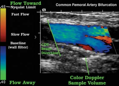 Figure 39.8. Color Doppler (CD) Image. This color Doppler image shows the bifurcation of the common femoral artery. The color map on the left side of the image shows red as the dominant color above the baseline indicating flow relatively toward the color Doppler beam direction. Blue is the dominant color below the color map baseline indicating flow relatively away from the color Doppler beam direction. Higher flow velocities are displayed in brighter colors transitioning to yellow in the “toward” direction and to green in the “away” direction. The CD sample volume is indicated in the image by an angled box (parallelogram). The orientation of the CD ultrasound beam is shown by the angled sides of the box. The mean Doppler shift is determined only within the box and is displayed in the appropriate color if flow is present. The background image is displayed in gray scale. |
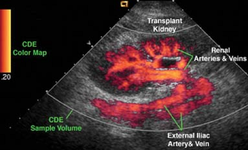 Figure 39.9. Power Doppler Image. This power Doppler image of a transplanted kidney nicely shows blood flow in the arteries and veins supplying the renal transplant as well as within the external iliac artery and vein. While power Doppler is highly sensitive to the presence of blood flow, it does not show the direction of flow. The shape of the power Doppler (CDE) sample volume is determined by the nature of the transducer used, in this case a sector transducer. |
On the CD image, flow directed toward the transducer is usually colored red whereas flow away from the transducer is usually colored blue. The operator may arbitrarily change the coloring of the Doppler information. The color map used is displayed as part of the color US image. Faster blood flow velocities are colored in lighter shades while slower blood flow is colored in darker shades. Color shading is dependent on mean velocities, not peak velocities. Thus, peak velocities cannot be estimated from the color image alone and must be determined from spectral Doppler. A normal laminar flow pattern will demonstrate lighter shades in the midstream and darker shades near the vessel walls, reflecting rapid flow in the middle of the vessel and slower flow near its walls. Disturbed flow, such as turbulence, is indicated by a wide range of colors in a scrambled pattern.
Changes in color within a blood vessel on a CD image may be caused by (1) change in the Doppler angle, (2) change in blood flow velocity, (3) aliasing, or (4) artifact. A change in Doppler angle causes a change in Doppler frequency shift, which, on a CD image, produces a change in the color displayed. Variations in the Doppler angle may be caused by the divergence of US beams emanating from sector or curved array transducers, a blood vessel curving through the color image, or a combination of both. CD images are used to detect changes in the blood flow velocity for further analysis by spectral Doppler. To interpret a CD image, inspect the color map for color display orientation, then analyze the image for variations in Doppler angle and blood flow velocity.
Doppler Artifacts. A variety of artifacts distort Doppler information and limit the information provided.
Aliasing is a limitation of pulsed Doppler US that occurs with both spectral and CD (3). Aliasing happens with high-velocity blood flow and improper velocity scale and baseline settings. Aliasing on spectral displays is seen as a “wrap-around” of peak velocities to the opposite end of the scale (Fig. 39.10). The highest velocities are cut off one side of the scale and artifactually displayed on the opposite side of the scale. Aliasing on CD “wraps-around” high velocities onto the opposite color scale (Fig. 39.11). For example, velocities too high for the red-scale setting are artifactually displayed as shades of blue. Color aliasing must be distinguished from true color changes caused by flow reversal or changes in the Doppler angle. True color changes are always surrounded by a black border, whereas color shifts related to aliasing lack this black border.
Aliasing occurs when the pulse Doppler sampling rate is too low for a given Doppler signal frequency, thus resulting
in an inaccurate frequency measurement. The US instrument measures the frequency of returning Doppler signal piece by piece by a series of pulses. The rate at which pulses can be transmitted (the pulse repetition frequency or PRF) is limited by the depth of the vessel interrogated. Deeper vessels require more time for the US beam to travel to the vessel and for the echo to return. To avoid aliasing, the PRF must be at least twice the frequency of the signal to be detected. The maximum frequency that can be accurately detected without aliasing is called the Nyquist limit and is equal to one-half the PRF. The Nyquist limit is displayed at the top and bottom of the spectral Doppler scale and the color map. On CD images, aliasing may be helpful and serve as a tag for high velocities associated with significant stenosis. Aliasing may be eliminated by proper adjustment of the Doppler scale and baseline settings, by using a lower Doppler transmission frequency, or by increasing the Doppler angle.
in an inaccurate frequency measurement. The US instrument measures the frequency of returning Doppler signal piece by piece by a series of pulses. The rate at which pulses can be transmitted (the pulse repetition frequency or PRF) is limited by the depth of the vessel interrogated. Deeper vessels require more time for the US beam to travel to the vessel and for the echo to return. To avoid aliasing, the PRF must be at least twice the frequency of the signal to be detected. The maximum frequency that can be accurately detected without aliasing is called the Nyquist limit and is equal to one-half the PRF. The Nyquist limit is displayed at the top and bottom of the spectral Doppler scale and the color map. On CD images, aliasing may be helpful and serve as a tag for high velocities associated with significant stenosis. Aliasing may be eliminated by proper adjustment of the Doppler scale and baseline settings, by using a lower Doppler transmission frequency, or by increasing the Doppler angle.
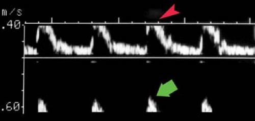 Figure 39.10. Aliasing on Spectral Doppler. The high velocity peaks of the spectral Doppler display are cut off at the top (red arrowhead), “wrapped around,” and displayed at the bottom (green arrow) of the spectral display. The spectral Doppler scale on the left is set with a Nyquist limit of 0.40 m/s, too low for the peak velocities encountered within the interrogated blood vessel. Aliasing in this case could be corrected by increasing the scale in the “toward” direction or by dropping the baseline. |
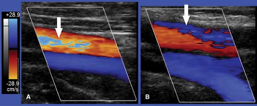 Figure 39.11. Aliasing Versus Flow Reversal on Color Doppler Imaging. The color map on the left shows that blue is the “toward” color and red is the “away” color. A. Aliasing. This image of the common femoral artery (in red) and vein (in blue) shows a patch of blue (arrow) in the femoral artery representing aliasing. Note that the blue in the artery is a light shade and that it is surrounded by a light shade of yellow. When the mean flow velocity exceeds the Nyquist limit, in this case 28.9 cm/s, aliasing occurs and the color display wraps around to the lightest colors on the opposite end of the scale, in this case from light yellow to light blue. The highest mean velocities in the femoral artery are aliased and displayed in light blue. B. Flow Reversal. In this image of the femoral artery and vein in the same patient but taken later in the cardiac cycle, normal reversal of flow (arrow) in early diastole is displayed in dark blue etched in black. True flow reversal goes through the baseline (shown on the image as the black border) and involves the darker color shades. |
Incorrect Doppler Gain. When the Doppler gain is set too low, Doppler information may be lost and blood flow may not be demonstrated. The CD image with too high gain demonstrates color in nonflow areas and random color noise. Correct gain settings are attained by turning up the gain setting until noise appears on the image and then slightly lowering the setting.
Velocity Scale Errors. Velocity range settings that are too high may obscure low-velocity flow, which is lost in noise and within the wall filter near the baseline. Vessels that are patent but with very slow flow may be considered thrombosed. When velocity scale settings are too low, aliasing occurs. Such aliasing is corrected by adjusting scale and baseline settings.
Color Flash. Any motion of a reflector relative to the transducer produces a Doppler shift (see Fig. 39.25). Rapid movement of the transducer itself may produce a Doppler shift and a flash of color projected over the gray-scale image. Most instruments incorporate motion discriminators that suppress color flash in hyperechoic but not in hypoechoic areas. Color flash is accentuated in cysts, the gallbladder, and other hypoechoic nonvascular structures. High color sensitivity settings accentuate color flash.
Tissue Vibration Artifact. Vibration of solid tissue may produce color display in perivascular tissues indicating flow where none is present. Tissue vibration artifact is produced in nonflow areas by bruits, arteriovenous fistulas, and shunts.
Fluid Motion. Color signal can be produced on CD images by motion of fluids other than blood. Motion of fluid within cysts and bowel may be misinterpreted as blood flow. Ureteral peristalsis produces a jet of color in the bladder that confirms patency of the ureter.
Carotid Ultrasound
Stroke follows heart disease and cancer as a leading cause of death in the United States. Stroke is caused by emboli from the heart or from unstable plaques in carotid vessels, or stenosis of the carotid arteries caused by extensive atherosclerotic plaque. The North American Symptomatic Carotid Endarterectomy Trial (NASCET) demonstrated significant benefit of endarterectomy in appropriate symptomatic patients with 70% to 90% stenosis of the ICA (10). The Asymptomatic Carotid Atherosclerosis Study showed the benefits of endarterectomy with reduced risk of stroke in asymptomatic patients with greater than 60% stenosis of the ICA (11). Carotid stenting and carotid angioplasty are additional treatments for carotid stenosis under investigation (12). Because of its accuracy, availability, and low cost carotid US competes effectively with MR and CT angiography for detection and classification of carotid disease (13).
Carotid Anatomy. The right common carotid artery (CCA) arises from the bifurcation of the innominate artery (14). The left CCA arises from the aortic arch. The CCAs ascend anterolaterally up the neck, medial to the jugular vein, and lateral to the thyroid. Each artery measures 6 to 8 mm in diameter. US of the CCA demonstrates the three layers of the normal vessel wall: the echogenic intima, hypoechoic media, and echogenic adventitia. The distance between these two echogenic lines (intima–media thickness) is normally less than 1 mm. The CCA dilates at the common carotid bulb and bifurcates near the angle of the jaw into the internal carotid artery (ICA) and the external carotid artery (ECA). The ECA usually (70%) assumes an anteromedial course off the carotid bulb. It overlaps the ICA in 20% of patients and is lateral to the ICA in 10%. The ECA has branch vessels that supply the head and face. It measures 3 to 4 mm in diameter. The ICA assumes a posterolateral course off the carotid bulb and measures 5 to 6 mm in diameter. The arterial wall between the ICA and ECA at their origin is the flow divider. The vertebral artery (VA) arises as the first branch of the subclavian artery, ascends in the transverse foramen of vertebrae C-6 to C-2, crosses the posterior arch of C1 to enter the foramen magnum, and forms
the basilar artery. Sonographic characteristics that aid in the differentiation of the ICA and ECA are listed in Table 39.3.
the basilar artery. Sonographic characteristics that aid in the differentiation of the ICA and ECA are listed in Table 39.3.
Table 39.3 Internal Carotid Artery Versus External Carotid Artery | ||||||||||||||
|---|---|---|---|---|---|---|---|---|---|---|---|---|---|---|
|
Technique. The American Institute of Ultrasound in Medicine provides guidelines for carotid US examination (15). Duplex US of the carotid arteries is performed with the patient in the supine position using a linear 5 to 10 MHz transducer. Higher frequency (>7 MHz) is used to assess plaque morphology and intima–media thickness. Lower frequency (<7 MHZ) is used for Doppler assessment (14). The patient’s head is rotated away from the side being examined. The cervical carotid arteries are evaluated in the longitudinal and transverse planes using gray-scale, color-flow, and spectral Doppler US. Atherosclerotic plaques are documented as to their extent, location, and characteristics (Fig. 39.12). CD is used to detect areas of narrowing and to select locations for spectral Doppler interrogation. Blood flow velocity measurements are documented at a minimum of 1 site in the CCA, ECA, and VA and two sites in the ICA (Fig. 39.13). Maximum PSV and diastolic velocity are recorded for both ICA. Direction of blood flow in each VA is recorded.
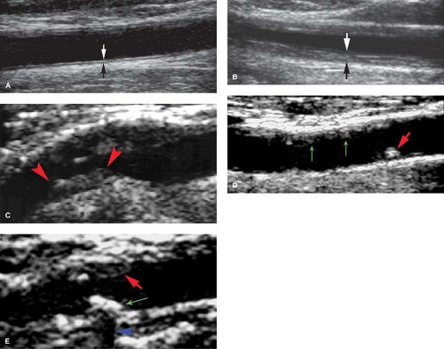 Figure 39.12. Plaque Evaluation. A. Normal Intima–Media Thickness. The normal thickness of the intima–media complex (between arrows) is less than 1 mm. The normal intima has a smooth well-defined luminal surface. B. Thickened intima–media complex (between arrows) is indicative of atherosclerosis and is associated with increased risk of stroke and ischemic heart disease. In this case, the intima–media complex measures 3 mm. C. Homogeneous plaque (arrowheads) has homogeneous echogenicity similar to that of muscle. D. Focal calcific plaque (short red arrow) and noncalcified plaque (long green arrows) produce an irregular luminal surface in the common carotid artery. E. Densely calcified plaque (long green arrow) causes an acoustic shadow (blue arrowhead) and homogeneous plaque (short red arrow) produces critical narrowing of the lumen at the origin of the internal carotid artery. |
Plaque Evaluation
Intima–media thickness is an index of the presence of atherosclerosis and a determinant of risk for stroke (Fig. 39.12) (16). The thickness of the echogenic intima and hypoechoic media is measured in the wall of the CCA, carotid bulb, and ICA. Normal thickness is less than 1 mm. Thickening greater than 1 mm is associated with aging as well as with increased risk of stroke and ischemic heart disease (17). Serial wall thickness measurements have been used to monitor the clinical response to specific treatments for atherosclerosis.
Plaque Formation. Carotid plaques are most commonly found within 2 cm of the bifurcation. Injury to the vascular endothelium results in the deposition of a fatty streak in the wall
of the artery. Plaque growth results from progressive deposition of lipids, proliferation of smooth muscle cells, and migration of fibrocytes. The “vulnerable” plaque contains a lipid core with a variable fibrous cap. As the plaque increases in size, the shearing forces of blood flow cause repeated episodes of fissuring and intraplaque hemorrhage with interval healing. During this process, the plaque can rupture causing cerebral emboli (18).
of the artery. Plaque growth results from progressive deposition of lipids, proliferation of smooth muscle cells, and migration of fibrocytes. The “vulnerable” plaque contains a lipid core with a variable fibrous cap. As the plaque increases in size, the shearing forces of blood flow cause repeated episodes of fissuring and intraplaque hemorrhage with interval healing. During this process, the plaque can rupture causing cerebral emboli (18).
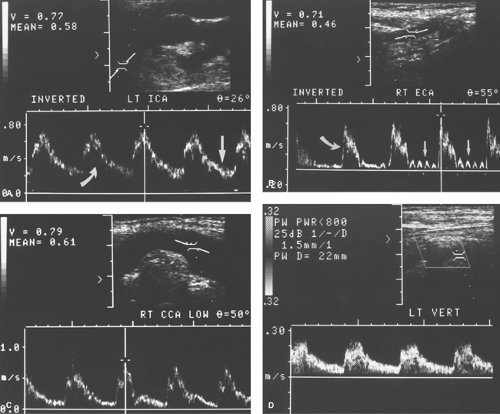 Figure 39.13. Normal Carotid Spectral Waveforms. A. Internal carotid artery (ICA)—low-resistance waveform. Note the prominent diastolic flow (arrow) and clean systolic window (curved arrow). B. External carotid artery (ECA)—high-resistance waveform. The rapid systolic upstroke is characteristic (curved arrow). The “sawtooth” pattern (arrows) is the result of the temporal tap. The sonographer palpates the pulse and then digitally taps either the superficial temporal or preauricular branch of the ECA. The tapping is transmitted back to the ECA as the “sawtooth” pattern on the spectral display. This maneuver helps distinguish the ECA from the ICA (no “sawtooth”) in difficult cases. C. Common carotid artery (CCA)—hybrid waveform. The CCA typically is more ICA-like since 70% of its blood flows into the ICA. D. Vertebral artery (VA)—low-resistance waveform. The VA often demonstrates spectral broadening due to its small size and location (poor visualization). Note the filling in of the systolic window with spectral broadening (curved arrow). |
Plaque Characterization. Plaques may be characterized as homogeneous or heterogeneous in US appearance (Fig. 39.12) (14). Homogenous plaques have a smooth contour and uniform internal architecture. They may be fibrous and soft or calcified and hard. Heterogeneous plaques contain intraplaque hemorrhage and increased amounts of lipid. They are fragile, unstable, may ulcerate, and are prone to embolize resulting in transient ischemic attacks, amaurosis fugax, and stroke. Ulcerated plaques show an irregular plaque surface on gray-scale US and eddy currents on CD (Fig. 39.14). All ulcerated plaques
are heterogeneous but not all heterogeneous plaques ulcerate. Plaque calcification is a nonspecific finding and is seen in both homogeneous and heterogeneous plaque (18). Densely calcified plaque may cause acoustic shadowing and block Doppler interrogation. Increasing evidence indicates that the identification of vulnerable plaque (heterogeneous and ulcerated plaque) in combination with biochemical markers of atherosclerotic disease may be useful in selecting patients for surgical, angiographic, and medical treatments for stroke prevention (19).
are heterogeneous but not all heterogeneous plaques ulcerate. Plaque calcification is a nonspecific finding and is seen in both homogeneous and heterogeneous plaque (18). Densely calcified plaque may cause acoustic shadowing and block Doppler interrogation. Increasing evidence indicates that the identification of vulnerable plaque (heterogeneous and ulcerated plaque) in combination with biochemical markers of atherosclerotic disease may be useful in selecting patients for surgical, angiographic, and medical treatments for stroke prevention (19).
Related posts:
Stay updated, free articles. Join our Telegram channel

Full access? Get Clinical Tree


