Vascular Ultrasound

Vascular US is based upon the use of the Doppler effect first described in 1842 by the Austrian mathematician Johann Christian Doppler. As applied to diagnostic US, the Doppler effect describes the change in sound frequency that occurs when sound is reflected from a moving object. In medical diagnostics, the US beam is reflected by clumps of moving red blood cells (RBCs) within blood vessels. The resulting change in sound frequency (the Doppler shift) is carefully measured to determine the presence, direction, and velocity of blood flow. Doppler shifts may also be produced by microbubbles induced by ureteral peristalsis producing a ureteral jet that confirms patency of the ureter. Doppler shifts produced by movement of the patient (breathing, heartbeat, and bowel peristalsis) or by movement of the transducer produces Doppler artifacts.

Understanding Doppler Ultrasound

The Doppler shift is the difference in sound frequency between the US beam transmitted into tissue and the echo produced by reflection from the moving RBCs. A Doppler interrogation beam is directed into tissue in a direction controlled by the operator. The Doppler beam intercepts moving blood within a blood vessel at an angle called the Doppler angle. Blood flow that is relatively toward the Doppler beam increases the frequency of the echo returning to the transducer (Fig. 11.1). The movement toward it compresses the Doppler sound wave. A “positive frequency shift” to a higher frequency indicates that blood flow is relatively toward the Doppler beam. A “negative frequency shift” to a lower frequency indicates that blood flow is relatively away from the Doppler beam. Doppler frequency shifts are fortuitously within the range of human hearing, so the sound of moving blood can be heard as well as measured by US.

The amount of frequency shift is proportional to the velocity of the moving RBCs. By using a mathematical formula (the Doppler equation) and the handy computer intrinsic to our US units, we can measure the Doppler shift and calculate blood flow velocity. It is most important to recognize that Doppler can accurately measure blood flow velocity, but is not
accurate at measuring blood flow volume. Measurement of blood flow volume requires accurate measurement of the cross-sectional area of blood vessels. This measurement is difficult and constantly changing because of the pulsatile nature of blood flow.

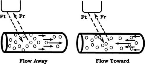Figure 11.1 Doppler Frequency Shift. Flow relatively away from the Doppler beam shifts the Doppler echo to a lower frequency. Flow relatively toward the Doppler beam shifts the Doppler echo to a higher frequency. Ft is the frequency of the transmitted Doppler beam. Fr is the frequency of the Doppler echo returned to the transducer.

The Doppler equation can be written in two ways:

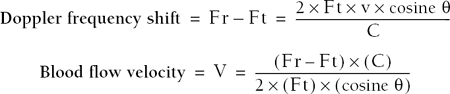
Ft is the frequency of the Doppler interrogation beam. Fr is the frequency of the echo shifted by the Doppler effect. (Fr – Ft) is the Doppler shift. C is the velocity of sound in human tissue, assumed to be constant at 1540 m/sec. V is the velocity of moving blood. The Doppler angle is indicated by the Greek letter theta (θ). The Doppler shift is proportional to the cosine function of the Doppler angle. The Doppler angle must be estimated by the operator and is communicated to the US unit by steering the “wing” of the Doppler angle indicator (Fig. 11.2).

For those mathematically inclined, the Doppler equation immediately demonstrates several important features of Doppler US. For those not mathematically inclined, just memorize the following facts:

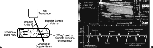Figure 11.2 Spectral Doppler Display. A. Drawing illustrates the Doppler beam, Doppler angle, Doppler sample volume, and the operator-controlled “wing” used to communicate to the US computer the estimated direction of blood flow. B. In this illustration, color Doppler and gray-scale US are used to locate and display the vessel being interrogated in the box at the top of the image. The spectral Doppler sample volume, the direction of the spectral Doppler US beam, and the Doppler angle indicator are shown. The Doppler spectrum is shown at the bottom of the image. See text for explanation of the spectral Doppler display (see Color Figure 11.2B).

Table 11.1: Cosine Values

Doppler Angle (θ)	Cosine Value
0°	1
10°	0.98
20°	0.93
30°	0.87
40°	0.77
50°	0.64
60°	0.50
70°	0.34
80°	0.17
90°	0

The Doppler frequency shift is the signal that we must optimize to obtain reliable blood flow velocity information. The Doppler signal is intrinsically weak, as little as 1/10,000 as strong as the gray-scale US signal. RBC reflectors in blood are very limited in number compared to innumerable sound reflectors within soft tissue. So, Doppler technique must always be optimized to produce useful and accurate information. The Doppler frequency shift is proportional to the Doppler transmission frequency. The higher the transmission frequency, the higher the Doppler shift. When blood flow velocity is slow, higher transducer frequency improves its detection. However, higher-frequency US is limited in penetration and lower frequencies must often be used to produce a Doppler signal from deep vessels.
The Doppler frequency shift is proportional to the cosine of the Doppler angle. This has important implications as seen by inspection of the cosine values listed in Table 11.1. The maximum Doppler frequency shift will be obtained by directing the Doppler interrogation beam straight down the barrel of the vessel—the Doppler angle is 0 degrees. The cosine of 0 degrees is 1, the maximum cosine value. Unfortunately, most blood vessels course parallel to the skin and a zero Doppler angle is seldom obtainable. The cosine of 90 degrees is zero. No Doppler shift is obtained at precisely 90 degrees of interrogation to direction of blood flow. In practice, a weak Doppler signal is often obtained because the Doppler interrogation beam diverges slightly. However, this weak signal is misleading as to flow direction and is inaccurate in determining velocity.
Acute Doppler angles (<60 degrees) must be created to obtain accurate Doppler information. Note from Table 11.1 that the cosine values change slowly at acute angles (10 degrees, 20 degrees) and change rapidly at larger angles (70 degrees, 80 degrees). The operator routinely assumes that blood flow is parallel to the walls of visualized blood vessels and aligns the Doppler angle “wing” to align with the wall of the vessel. However, blood vessels, especially diseased arteries, are commonly tortuous and the exact orientation of blood flow and the Doppler angle must be estimated. Erroneous estimates of the Doppler angle cause smaller errors in blood flow velocity calculations at acute angles than at angles close to 90 degrees. The Doppler shift diminishes to 50% of maximum at 60 degrees, and falls rapidly at larger angles, reducing the quality of Doppler information. A 60 degrees, or smaller, Doppler angle is obtainable, with effort, in nearly all imaging situations.

Continuous wave (CW) Doppler uses two US crystals, one as a transmitter and the other as a receiver, to continuously record all Doppler shift information along the entire path of the Doppler beam. CW Doppler is non-selective and combines all Doppler shift information from all blood vessels in its path. CW Doppler is used commonly in obstetrics to monitor fetal heart tones.

Pulsed wave Doppler is commonly used in conjunction with real-time gray-scale US imaging to perform duplex Doppler US. Duplex Doppler combines routine imaging with Doppler interrogation of visualized vessels. Excluding all signals obtained along the Doppler
beam line-of-sight except those obtained from a small time window creates a Doppler sample volume (Fig. 11.2A). This sample volume can be precisely positioned within any vessel visualized to obtain selective blood flow information from one vessel or even just a portion of one vessel. The combination of gray-scale US, color Doppler, and spectral Doppler is sometimes called triplex Doppler US (Fig. 11.2).

Spectral Doppler displays Doppler shift information as a graph of velocity, or frequency shift, information displayed over time. Blood flow velocity can be displayed interchangeably with Doppler frequency shift information by solving the Doppler equation shown previously. The appearance of the Doppler spectrum remains the same; only the scale changes.

Color Doppler uses a larger sample volume to detect mean Doppler shifts within a larger visualized area. Moving blood is displayed in color superimposed upon the gray-scale image.

Doppler Spectral Display

Echoes returning from the Doppler sample volume are analyzed for frequency shift information. A Fast Fourier Transform sorts the range and mixture of Doppler shift information into individual components and displays them as a function of time. Analysis is performed rapidly enough to display the information in real time corresponding to heartbeat (Fig. 11.2B).

The horizontal scale (x-axis) is time in seconds.
The vertical scale (y-axis) is flow velocity in m/sec or cm/sec, or is the Doppler frequency shift in kHz.
Brightness of pixels in the spectrum corresponds to the relative number of RBCs moving at given velocity at a specific instant in time. The more RBCs moving at that specific velocity and time, the brighter the pixel.
Flow relatively toward the Doppler beam is displayed above the zero baseline.
Flow relatively away from the Doppler beam is displayed below the zero baseline.
Spectral waveforms vary over time with cardiac contraction with highest flow velocities during systole and lowest flow velocities during diastole. Many vessels show reversed flow or no flow during diastole.

Color Doppler Imaging Display

Color Doppler imaging (CDI) superimposes Doppler flow information on a standard gray-scale real-time US image. Color Doppler displays colors based on measurement of mean Doppler shifts (Fig. 11.3) [1].

A color map is displayed adjacent to the image to indicate the colors used to display flow information [2]. A wide variety of color maps are available. The map in use must be analyzed to interpret the color information (Fig. 11.4).
The color map is divided into two parts by a black bar that corresponds to the baseline or zero flow point on the Doppler spectral display. The color on the top of the map, above the baseline, is used to show flow relatively toward the Doppler beam. The color on the bottom of the map, below the baseline, shows flow relatively away from the Doppler beam. Red is commonly used to indicate flow toward the Doppler beam, whereas blue indicates flow away from the Doppler beam. Obviously, red and blue colors provide no direct indication of whether vessels are arteries or veins. Knowledge of anatomy, appearance of the vessel, and Doppler waveform analysis are used to differentiate various arteries and veins.
Brighter colors are used to display higher mean velocities. Darker colors indicate lower mean velocities. Some color maps use different color shades for higher and lower velocities (Fig. 11.3). For instance, red may transition to yellow and blue may transition to green for higher flow velocities.
Numbers at the top and bottom of the color map indicate the velocity scale setting the Nyquist limit. The velocity scale must be set appropriately to the blood flow velocity
encountered. A scale set too high will obscure slow flow. A scale set too low will alias. Aliasing and the Nyquist limit are discussed later in this chapter.
A color Doppler sample volume is specified and positioned on the gray-scale image by the US operator. The color Doppler sample volume box is usually etched in white. Only the tissue within the box will be analyzed for Doppler shift information. Keeping the sample volume small optimizes Doppler information gathering.
Note that in CDI the format of the transducer determines the direction of the Doppler beam. The Doppler angle may change with vessel orientation and produce color changes related only to changes in the Doppler angle and not to changes in blood flow.
As with spectral Doppler, color flow information will not be obtained when the Doppler angle is at or near 90 degrees.
The color displayed within blood vessels on CDI is a function of
- – Flow velocity
- – Doppler angle
- – Presence of aliasing
- – Color map utilized
- – Phase of the cardiac cycle

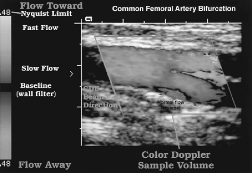Figure 11.3 Color Doppler Imaging Display. The color map is shown on the left side of this image. See text for detailed explanation of the color Doppler display (see Color Figure 11.3).

Color Doppler and spectral Doppler are complementary to each other. Color flow shows flow information based on measurement of mean Doppler shifts, whereas spectral Doppler displays the full range of detected Doppler shifts. Color flow imaging can be used to detect blood vessels and confirm presence and direction of blood flow, whereas spectral Doppler provides more detailed characterization of blood flow and precise velocity measurements to estimate stenosis.

Color Doppler Energy Display

Color Doppler energy (CDE) displays color flow information obtained from integration of the power of the Doppler signal, rather than the Doppler frequency shift itself [3]. Another name for this technique is power Doppler. CDE relates more directly to the number of moving
RBCs than to their velocity. CDE is relatively angle-independent and is more sensitive to slow flow than is CDI. CDE is a useful adjunct to CDI, especially in technically challenging situations. CDE significantly improves evaluation of parenchymal flow and assessment of tumor vascularity (Fig. 11.5) [4, 5].

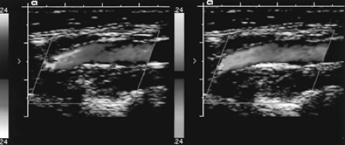Figure 11.4 Color Maps. Inversion of the color map radically changes the appearance of the color image of a carotid artery. Choice and orientation of the color map are at the option of the US operator (see Color Figure 11.4).

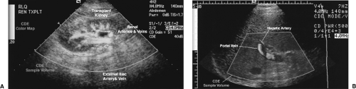Figure 11.5 Color Doppler Energy Display. A. The blood vessels within and supplying a renal transplant are displayed on this color Doppler energy (CDE) (power Doppler) image. CDE shows the presence of blood flow with high sensitivity. However, direction of blood flow is not determined and adjacent arteries and veins with blood flow in opposite directions are shown in the same color. The CDE sample volume is adjusted by the operator to include the tissues of interest. B. CDE image of the liver shows flow in the portal vein and hepatic artery. In this example, the Doppler sample volume is shaded in color (see Color Figure 11.5).

CDE provides no information on flow direction or velocity.
Artifacts related to patient motion are significantly increased with CDE compared to CDI. Patients unwilling or unable to hold their breath or remain motionless may not be accurately imaged with CDE.
Visualization of gray-scale anatomy is often limited within the CDE sample volume.
CDE also displays a color map adjacent to the image. As with CDI, the colors chosen are arbitrary. However, no information on flow direction is obtained with CDE.
The CDE sample volume may be shaded in a color different than that used to indicate blood flow.

Blood Flow Dynamics

The major types of blood flow are laminar (parabolic), plug, disturbed, and turbulent [6].

Laminar Blood Flow

Laminar blood flow is the normal blood flow found in arteries and in large veins (Fig. 11.6) [7]. The highest velocity RBCs are in the center of the blood vessels. Blood flow velocity progressively decreases closer to the vessel wall. Blood at the vessel wall is hardly moving. Laminar blood flow is sometimes called parabolic blood flow because a line connecting the levels of flow at differing velocities has the shape of a parabola. The characteristics of laminar flow are:

Spectral Doppler shows a narrow range of velocities within the sample volume at any given instance in time. This is the normal “narrow spectrum” (Fig. 11.6B).
A well-defined window is seen beneath the Doppler spectrum in systole reflecting the fact that detected RBCs accelerate uniformly during systole. This is called the “systolic window.”
Highest flow velocities are mid-stream with decreasing flow velocities closer to the vessel wall.
Color Doppler shows the brightest color mid-stream with darker colors toward the vessel wall (Fig. 11.6C).
Cardiac contraction causes flow velocity to increase rapidly to peak values during systole, then flow velocity decreases with diastole during which there may be no flow or flow may reverse in direction.
The sound of laminar flow has a whistling quality.

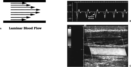Figure 11.6 Normal Laminar Blood Flow. A. Arrows represent the orderly layers of red blood cells moving at different velocities that characterize laminar blood flow. The highest velocities are found in mid-stream. The lowest velocities are found adjacent to the vessel wall. B. Doppler spectral display shows the narrow spectrum characteristic of laminar flow in the common femoral artery. The systolic window (arrow), characteristic of laminar flow, is seen as the triangular space beneath the Doppler spectrum in systole. C. Color Doppler image of the common carotid artery at mid-systole shows bright color in mid-stream, indicating faster flow, and darker color near the vessel wall, indicating slower flow (see Color Figure 11.6C).

Plug Flow

Plug flow is a type of normal flow seen in large diameter vessels such as the aorta. In mid-stream a wide band of RBCs is moving at the same speed, forming a plug-shaped velocity profile.

The Doppler spectral is very narrow, reflecting RBCs all moving at the same speed throughout the cardiac cycle.

Disturbed Blood Flow

Disturbed blood flow occurs at vessel bifurcations and in areas of vessel stenosis. Disturbed flow no longer travels in a straight line but generally continues in a forward direction [8].

Flow velocity is increased (Fig. 11.7).
“Spectral broadening” indicates the disorganization characteristic of disturbed flow. The thickness (vertical height) of the Doppler spectrum is increased, indicating a broader range of the velocities within the sample volume at any given instant of time.
Increased spectral broadening indicates increased disturbance of flow. The systolic window characteristic of laminar flow is reduced in size and may be obliterated.

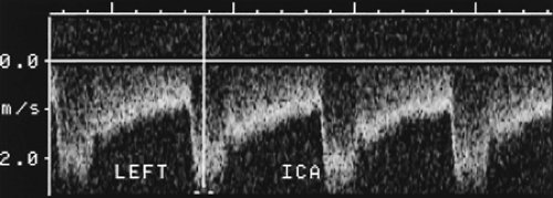Figure 11.7 Disturbed Blood Flow. Spectral display of the waveform obtained in an area of high-grade stenosis of the internal carotid artery (ICA). Peak systolic velocity is increased to 270 cm/sec. The spectrum is broadened and ill-defined.

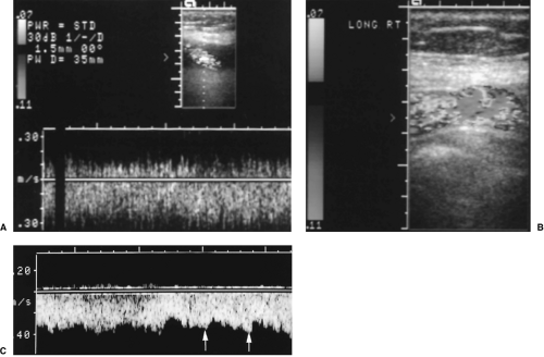Figure 11.8 Turbulence. Severe turbulence within a venous shunt is seen on spectral Doppler, A, and on color Doppler, B. C. Marked turbulence downstream from a severe renal artery stenosis shows marked spectral broadening and a waveform that is barely recognized as pulsatile. The arrows indicate systolic peaks (see Color Figure 11.8B).

Turbulent Blood Flow

Turbulent blood flow is random and chaotic, with RBCs flowing in all directions. Turbulence is found downstream from high-grade stenosis and in areas where flow velocities are very high, such as within shunts and fistulas [8].

Spectral broadening is severe and the systolic window is obliterated (Fig. 11.8A).
With severe turbulence, flow is concentrated at lower velocities.
With severe stenosis, flow is less pulsatile.
Flow may be detected in both directions simultaneously, owing to the formation of eddy currents. Eddy currents occur downstream from high-grade obstructions where the blood vessel lumen widens after the stenosis.
Flow velocities fluctuate with time.
Color Doppler shows a mixture of colors with aliasing reflecting the high velocities (Fig. 11.8B).

Individual blood vessels may be characterized by their Doppler “signatures,” a recognizable Doppler spectrum relatively unique to the vessel (Fig. 11.6B). A major determinant of the appearance of the Doppler spectrum is downstream resistance to blood flow. Blood vessels may be characterized as being “high resistance” or “low resistance” vessels.

High Resistance Blood Vessels

When vessels show a high resistance pattern, small arteries and arterioles downstream are contracted, increasing resistance to blood flow and maintaining blood pressure at high
levels. Pulse pressures traveling down the arterial tree are highly reflected resulting in little flow to the capillary bed during diastole. Arteries that supply systemic muscles are characteristically high resistance when the muscles are at rest. With exercise, arterioles open, blood flow increases, and the high resistance pattern converts to low resistance.

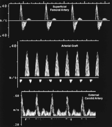Figure 11.9 High Resistance Spectra. Triphasic high resistance patterns are shown in the spectra of the superficial femoral artery and an arterial graft. The external carotid artery shows a relatively high resistance pattern with low velocity flow in diastole.

A triphasic waveform characterizes arteries supplying skeletal muscles at rest (Fig. 11.9). Examples include the femoral artery, the external iliac artery, and the radial artery.
- – Velocity rises sharply with onset of systole and falls rapidly with cessation of ventricular contraction.
- – Flow reverses for a short time in early diastole.
- – The remainder of diastole shows little or no forward flow.
Some arteries show relatively high resistance patterns. Examples include the external carotid artery (ECA) (Fig. 11.9) and the superior mesenteric artery (SMA) during fasting.
- – The rise to peak systolic velocity (PSV) is sharp with a rapid fall of velocity at the termination of systole.
- – Flow in diastole remains forward in direction but is at very low velocity.

Low Resistance Blood Vessels

Low resistance blood vessels are characterized by forward flow throughout the cardiac cycle. These arteries supply vital organs like the brain and kidneys that demand a continuous supply of oxygenated blood. Arterioles within these organs are generally kept wide open.

Low resistance arteries have characteristic biphasic waveforms. Examples include the internal carotid artery (ICA), the renal artery, the umbilical artery, and the SMA after eating (Fig. 11.10).
- – Velocity rises more slowly and falls more gradually during systole.
- – Flow is forward throughout the cardiac cycle.
- – Flow never reaches the zero velocity baseline.

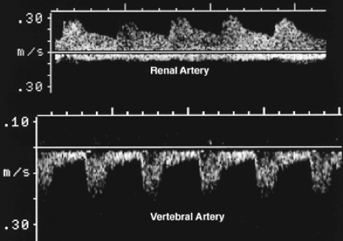Figure 11.10 Low Resistance Spectra. The renal artery and vertebral artery show relatively high velocity flow in diastole characteristic of low resistance spectra seen in arteries that supply vital organs. Forward flow toward the organ is present throughout the cardiac cycle.

Velocity Ratios

Many times a Doppler signal can be obtained from tiny blood vessels that cannot be discretely visualized. Intrarenal arteries are a common example. At other times the vessel is so tortuous that a Doppler angle cannot be accurately estimated, such as in the twisted umbilical artery in the umbilical cord. Without an accurate Doppler angle estimation, an accurate flow velocity cannot be determined. In these instances the Doppler equation can be solved using the measured Doppler frequency shift and a cosine θ value of 1. The velocity values will not be accurate, but the Doppler spectrum characterizes flow within the blood vessel. A variety of velocity ratios can be calculated from the displayed Doppler spectrum. The formulas for the commonly used velocity ratios are displayed in Box 11.1.

Resistance index is also called the Pourcelot index. It is calculated by subtracting end diastolic velocity from PSV and dividing the result by PSV. A high resistance index indicates high resistance to blood flow within the vessel. High resistance to blood flow may be produced by arteriole constriction or by limited arterial distensibility such as may be produced in an edematous obstructed kidney [9].
Systolic/diastolic ratio (A/B ratio) is calculated by dividing PSV by end-diastolic velocity.
Pulsatility index requires determination of temporal mean velocity and thus is more difficult to calculate. US computers allow the operator to trace the spectrum and the computer will calculate a mean velocity (Fig. 11.11). Pulsatility index is then calculated by subtracting end diastolic velocity from PSV and dividing the result by mean velocity.

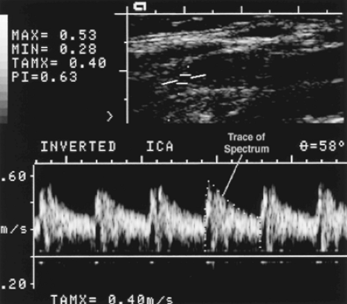Figure 11.11 Pulsatility Index. The operator manually traces the outline of one cardiac cycle on the Doppler spectrum. From this tracing, the US computer determines the temporal mean velocity and calculates the pulsatility index (PI). The result is displayed in the upper left-hand corner of the image (PI = 0.63). ICA, internal carotid artery.

Doppler Changes Caused by Stenosis

A common use of Doppler US is to detect and characterize arterial stenosis. Gray-scale US will identify atherosclerotic plaques and vessel narrowing. The severity of stenosis is determined by correlation of Doppler findings with real-time imaging.

Proximal to the stenosis, laminar flow is generally present unless the vessel is seriously diseased upstream (Fig. 11.12).
Within the stenotic zone, flow velocity is increased but usually remains laminar. PSV correlates best with the severity of stenosis. The highest velocity may be found in a very small region of the stenosed vessel lumen. A careful search of the vessel with a small sample volume is needed.
In the post-stenotic zone, spectral broadening occurs as flow spreads out to occupy the widened vessel lumen. Turbulence and eddy currents form downstream to severe stenosis. Maximum flow disturbance is usually found within 1 cm of the maximum stenosis.
Downstream, the Doppler signal is dampened by severe stenosis. This results in the tardus parvus waveform.

Tardus Parvus Waveform

The tardus parvus waveform is a sign of marked arterial stenosis that does not require direct evaluation of the stenosis [10]. The waveform is detected in arteries downstream from the
stenosis. It is particularly useful in situations where visualization of the supplying artery is commonly difficult because of location of the artery or obscuration by bowel gas. Evaluation for stenosis of the renal artery or stenosis of an artery supplying a transplant are examples (Fig. 11.13) [11].

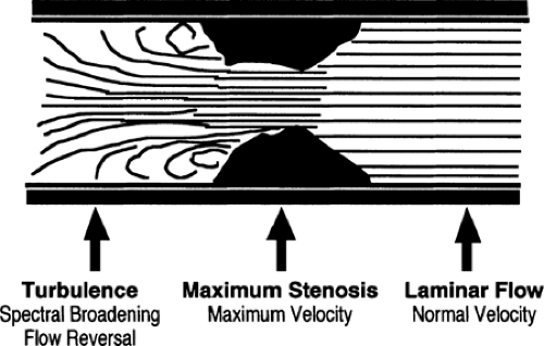Figure 11.12 Velocity Changes Across a Vessel Stenosis. To maintain flow volume across an area of stenosis, velocity must increase through the stenotic segment. The maximal change in velocity occurs at the site of greatest narrowing. Doppler velocity measurements made at this site correlate best with the severity of stenosis. Beyond the stenosis, flow is disturbed and sampling shows spectral broadening, turbulence, and areas of flow reversal.

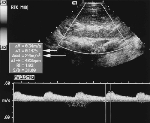Figure 11.13 Tardus Parvus Waveform. Doppler of an intrarenal artery in a patient with surgically proven, renal artery stenosis shows a characteristic tardus parvus waveform. The acceleration time (δT) (short arrow) is 0.142 seconds. The acceleration index (Accl) (long arrow) is 2.4 m/sec2. Note the blunted appearance of the waveform in systole.

Tardus refers to a slowed systolic upstroke. This can be measured by acceleration time, the time from end diastole to the first systolic peak. An acceleration time >0.07 sec correlates with >50% stenosis of the renal artery [12].
Parvus refers to decreased systolic velocity. This can be measured by calculating the acceleration index, the change in velocity from end diastole to the first systolic peak. An acceleration index <3.0 m/sec2 correlates with >50% stenosis of the renal artery [12].

Venous Flow

Blood flow within veins is typically low velocity and non-pulsatile. However, venous spectra may be phasic when influenced by respiration, may vary in velocity when influenced by motion of the vein itself, or may be pulsatile when transmitting motion from the right side of the heart. These normal variations in venous flow must be recognized to avoid diagnostic errors (Fig. 11.14).

Portal Vein

The portal vein is formed by the confluence of the splenic and superior mesenteric veins. It provides approximately 70% of the incoming blood to the liver.

Normal blood flow velocity is 13-23 cm/sec with an average of 18 cm/sec.
Flow velocity is commonly somewhat phasic because rocking motion of the liver caused by motion of the heart moves the portal vein under the Doppler sample volume (see Fig. 11.24).
Slight phasicity may also be evident related to respiration.
Normal blood flow direction is into the liver. Any reversal of blood flow direction is abnormal and usually indicative of portal hypertension.
The portal vein is normally <13 mm in diameter. Increased diameter suggests portal hypertension.

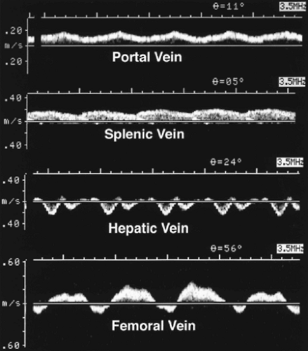Figure 11.14 Venous Waveforms. Doppler spectra from the portal, splenic, hepatic, and femoral veins are shown. See text for discussion of the waveforms.

Splenic Vein

The splenic vein drains the spleen and receives inflow from the inferior mesenteric vein. The splenic vein joins the superior mesenteric vein posterior to the neck of the pancreas to form the portal vein.

The splenic vein shows low velocity forward flow toward the liver. Reversal of blood flow direction is seen with advanced portal hypertension.
Slight respiratory variation is common.
Normal diameter of the splenic vein is <10 mm. Increase in diameter is a sign of portal hypertension.

Hepatic Veins

Most individuals have three major hepatic veins that run a straight course to converge in the inferior vena cava just below the diaphragm and only approximately 1 cm from the right atrium. These three hepatic veins drain all of the liver except the caudate lobe. The appearance of the right, middle, and left hepatic veins and inferior vena cava has been likened to a Playboy bunny, a crow’s foot, or a caribou with antlers.

Pulsations of the right atrium are transmitted directly to the inferior vena cava and hepatic veins. None of these veins contains valves.
The normal hepatic vein waveform is undulating and mirrors motion of the right heart. The A-wave (reversed flow) is produced by atrial contraction. Forward flow of atrial filling is interrupted by the C-wave caused by bulging of the tricuspid valve with onset of ventricular contraction. The dominant S-wave represents high velocity atrial filling during ventricular systole. The V-wave represents the end of atrial filling and the D-wave is produced by opening of the tricuspid valve and simultaneous filling of the right atrium and right ventricle.
Color Doppler accurately demonstrates the normal flow direction changes characteristic of the hepatic vein (Fig. 11.15).

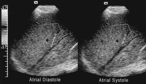Figure 11.15 Normal Hepatic Vein Flow. Blood flow in the hepatic veins is normally toward the heart during atrial filling and away from the heart during atrial contraction. Note that a static color Doppler image represents only an instant in time during the cardiac cycle. Compare to the hepatic vein waveform in Figure 11.14 (see Color Figure 11.15).

Peripheral Veins

Venous flow from the extremities occurs in response to the effects of gravity and muscular contraction.

Blood flow in peripheral veins is low velocity and may be appear to be absent if the Doppler velocity scale is set too high or if a large wall filter is used (see Fig. 11.21).
Flow shows respiratory variation (Fig. 11.14) caused by changes in intra-abdominal pressure produced by motion of the diaphragm. With inspiration the diaphragm descends, increasing intra-abdominal pressure and decreasing venous flow from the legs. With expiration the diaphragm rises, intra-abdominal pressure decreases, and venous flow from the legs increases. If the patient holds his breath, venous flow usually stops. A Valsalva maneuver will reverse flow in the lower extremity veins. Squeezing the patient’s calf will augment flow and improve detection of veins.

Doppler Artifacts

Artifacts produce confusing alterations of the Doppler signal and affect both spectral Doppler and color flow imaging. Artifacts are produced by physical limitations of Doppler instrumentation and by incorrect instrument settings [13]. Recognition of artifacts and proper correction prevents misdiagnosis.

Aliasing

Aliasing is a performance limitation of pulsed Doppler US that is related to the pulse repetition frequency. Pulse repetition frequency is limited by depth. The greater the distance to the vessel of interest, the longer it takes to transmit and receive echoes from that vessel. The Doppler signal that must be measured is the echo of the transmitted Doppler pulse that has been changed in frequency by reflection from moving RBCs. To accurately measure the frequency of the Doppler echo, the pulse repetition frequency must be at least twice the frequency of the Doppler echo. For any given setting of the Doppler US instrument, the Nyquist limit is defined as the maximal Doppler shift frequency that can be accurately measured. Because Doppler shift frequency and blood flow velocity can be substituted for each other mathematically by use of the Doppler equation, the Nyquist limit can also be expressed as the maximal blood flow velocity that can be detected by Doppler for a given set of instrument settings.

Aliasing produces a wrap-around effect on the Doppler display. On spectral Doppler, the peaks of the spectrum are cut off and displayed on the opposite side of the baseline (Figs. 11.16, 11.17).
On color Doppler, aliasing projects the color of reversed flow within central areas of highest velocity (Fig. 11.18). The key to recognizing color aliasing is to observe that no black stripe surrounds the color change. Color change of aliasing involves the brightest
shades of the color display. Color change produced by true reversal of blood flow direction, or by changes in the Doppler angle, are etched in black and involve the darkest shades of the color display.
On most Doppler instruments the pulse repetition frequency cannot be adjusted directly.
Increasing the velocity scale, which increases the pulse repetition frequency, can eliminate aliasing. Changing the baseline setting or using a lower Doppler US frequency can also eliminate aliasing.
Aliasing is not a feature of CDE (power Doppler) [14].

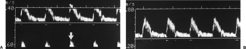Figure 11.16 Aliasing in Spectral Doppler. A. Spectral Doppler shows the peaks (curved arrow) of the spectral display are cut off the top and are displayed on the bottom (straight arrow). B. With readjustment of the baseline to allow display of the 80 cm/sec peak systolic velocity, the aliasing is eliminated.

Spectral Broadening

Spectral broadening is an important spectral Doppler sign of abnormal blood flow. However, spectral broadening has a number of other causes that must be recognized and excluded before spectral broadening can be interpreted as a sign of abnormal blood flow.

When the Doppler sample volume is large compared to the size of the blood vessel, the sample volume will include the full range of blood flow velocities from slow flow near the vessel wall to the fastest flow in midstream. Inclusion of all flow velocities will broaden the spectrum. Because the smallest sample volume available on most Doppler instruments is 1.0-1.5 mm, vessels of this size and smaller will inevitably show broadening of the displayed velocity spectrum.
Placing the sample volume near the vessel wall instead of mid-stream will produce spectral broadening by inclusion of the slow-moving RBCs near the vessel wall. The highest flow velocities in mid-stream may be missed.
Excessive Doppler gain falsely broadens the spectrum.

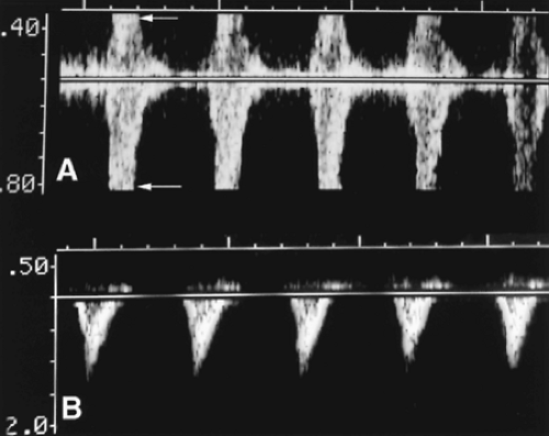Figure 11.17 Aliasing in Spectral Doppler. A. In an example of more severe aliasing, both the top and bottom (arrows) of the spectrum are cut off. Direction of blood flow cannot be determined from this spectrum. B. Adjustment of baseline and scale results in appropriate display of the spectrum.

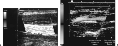Figure 11.18 Aliasing in Color Doppler. A. The dominant color displayed within this vessel is yellow from the top side of the color map. Yellow indicates flow toward the Doppler beams, or in this case, from right to left. The splotches of green color are areas of aliasing. Note the absence of a black border. The color velocity scale is set low with a Nyquist limit of 0.040 m/sec. When the detected mean blood flow velocity exceeds this limit, aliasing occurs and color from the bottom portion of the color map is displayed. Aliasing must be recognized, but in this case may be useful by providing identification of highest velocity flow. B. This color Doppler image of the internal carotid artery demonstrates the appearance of true reversal of blood flow direction as indicated by the black border around the region of color shift. A small area of flow reversal is a normal finding opposite the flow divider at the bifurcation of the common carotid artery. Note that the direction of the Doppler beams is different than the direction of the gray-scale image beams (see Color Figure 11.18).

Incorrect Doppler Gain

When the color or spectral Doppler gain is set too low, Doppler information may be lost and blood flow may not be detected. The color image with gain set too high demonstrates color in non-flow areas and random color noise. Correct gain settings are attained by turning up the gain setting until noise appears on the color image or spectral display, then gain is reduced slowly until the noise disappears.

Gain set too low shows no spectral display or color flow on the image.
Color gain set too high shows color bleed beyond the limits of the vessel, color signal in non-flow areas, and random color noise.
Spectral gain set too high shows random noise on the spectral display, false spectral broadening, and commonly displays a mirror image of the spectrum on the opposite side of the baseline (Fig. 11.19).

Velocity Scale Errors

Errors in the setting of the Doppler velocity scale may obscure slow flow or cause aliasing. Velocity scale and baseline settings must be adjusted to be appropriate to the velocity of blood flow in the interrogated vessel.