,  ) of our template vertebra were selected. These two points allow to compute the centre of the vertebral body (VB) as well as the direction from
  to
to  (
( ) of each initial vertebra.
In the segmentation step, the intervertebral discs (IVD) centres were manually pinpointed. From these points, the new VB centres were computed as the mean point between two consecutive IVD centres, with the exception of the L1, which was extrapolated from the other points. The scaling factor ( ) and the rotation matrix (R) were computed as:

where ( ) is the vector that goes from the IVD below the vertebra to the IVD on the top,
  defines the dot product between
  and
and  .
.  was set to 0.9 and it was used to compensate the difference between the endplate landmarks and the distance between two consecutive IVDs.
 ) and the rotation matrix (R) were computed as:
(1)
 ) is the vector that goes from the IVD below the vertebra to the IVD on the top,
  defines the dot product between
  and
and  .
.  was set to 0.9 and it was used to compensate the difference between the endplate landmarks and the distance between two consecutive IVDs.
2.2 Vertebra Segmentation
The algorithm follows our previous work [4], where a set of features and weights ( ) were trained. For this task, the training database (Sect. 2.3) was used. Vertebrae were divided into two regions (see Fig. 1), the articular processes (AP) and the rest (RV). Three features were trained for each region, for the RV: The oriented derivative from high to low intensity, the intensity itself and the distance from the current position were used. For the AP, the same features were employed but the first one, which was exchanged for a feature more adequate to the space between the articular processes. This feature seeks a sudden decrease of intensity followed by an increase of it. Thus, the cost functions are:


where  is the current position of the mesh point
  ,
,  is a vector, whose values are the intensity profile positions in the image along the normal direction of the mesh surface at point
  ,
,  is the normal direction at
  from inside to outside of the mesh,
  is the image intensity,
  represents the euclidean distance from
  to
to  and
and  represents the convolution of a set of filter F and the profile of intensities. F is in the form of [1’s, 0’s,
  1’s, 0’s, 1’s], where the length (
 ) of the components are variable.
 ) were trained. For this task, the training database (Sect. 2.3) was used. Vertebrae were divided into two regions (see Fig. 1), the articular processes (AP) and the rest (RV). Three features were trained for each region, for the RV: The oriented derivative from high to low intensity, the intensity itself and the distance from the current position were used. For the AP, the same features were employed but the first one, which was exchanged for a feature more adequate to the space between the articular processes. This feature seeks a sudden decrease of intensity followed by an increase of it. Thus, the cost functions are:
(2)

(3)
 is the current position of the mesh point
  ,
,  is a vector, whose values are the intensity profile positions in the image along the normal direction of the mesh surface at point
  ,
,  is the normal direction at
  from inside to outside of the mesh,
  is the image intensity,
  represents the euclidean distance from
  to
to  and
and  represents the convolution of a set of filter F and the profile of intensities. F is in the form of [1’s, 0’s,
  1’s, 0’s, 1’s], where the length (
 ) of the components are variable.
Stay updated, free articles. Join our Telegram channel

Full access? Get Clinical Tree


