Vertebra Segmentation from MR Dixon for Hybrid Whole-Body PET/MR

Fig. 1

Segmentation model and segmentation pipeline. a The model compartments being used for model localization (based on the generalized Hough transform). b Parametric adaptation. Individual affine transformations are assigned to the “anchoring structures” femur/pelvis/lungs. The vertebrae are deactivated in this step (transparent) to avoid wrong mesh to image vertebra assignments. All vertebrae are positioned according to the remaining components. c Deformable adaptation. In this final step, the segmentation is refined using local mesh deformations. All vertebrae are consecutively activated and adapted to the image (from sacrum to neck) to ensure correct vertebra labelings

The surface model being used as shape prior for segmentation is shown in Fig. 1a. Since a direct vertebra segmentation from whole-body images is prone to localization errors, we choose a combined model that includes tissues that serve as “anchoring strucures” for the vertebrae: (1) femur/pelvis and (2) lungs. Note that both femur and pelvis were chosen as anchoring structures in the pelvic region because they showed most reliable segmentation results due to clear image deliniations between bone and soft tissue. In other words, we first segment femur/pelvis/lungs to initially place the vertebrae at their approximate position (i.e. within the capture range), before they are locally adapted to the image. The segmentation pipeline consists of three steps (see [10] for details):

Step 1. Model localization. In this first step, the model is located in the image at the approximately correct position. The localizer is based on the generalized Hough Transform (GHT) and attempts to align mesh triangles with image gradients. Step 2. Parametric adaptation. Multiple rigid/affine transformations of the anchoring structures (different colors in Fig. 1b) allow registration of these structures with the image. In this step all vertebrae are deactivated (transparent in Fig. 1b) to avoid wrong anatomical correspondences between mesh and image vertebra. They are rather passively scaled and positioned at their approximate location in the image based on the transformations of the anchoring structures. Step 3. Deformable adaptation. In this final step, first all anchoring structures are simultaneously adapted to the image using local deformations. The vertebrae are then successively activated (from sacrum to neck) to ensure a correct localization of each individual vertebra: first the lumbar vertebra 5 is activated and adapted to the image, then the next lumbar vertebra 4 is activated and adapted, then lumbar vertebra 3, etc. (Fig. 1c). This iterative activation and adaptation is repeated until the top thoracic vertebra 1 is reached.

2.2 Multi-modal Features

Fig. 2

Target point detection using multi-modal image features. For each mesh triangle, a search profile is defined along the perpendicular triangle direction. Target points $x^{water}$ and $x^{fat}$ are detected as the one points that maximize a feature response (such as the maximum image gradient) in the water (a) and in the fat image (b), respectively. During adaptation, the mesh triangle is simultaneously attracted to $x^{water}$ as well as to $x^{fat}$

During parametric as well as during deformable adaptation, the mesh triangles are attracted to image target points detected by the following algorithm (Fig. 2). For each mesh triangle, we construct a search profile (perpendicular to the triangle) of

points

with $i\in [-l, l]$ and search for a target point that maximizes an image feature response

$\begin{aligned} x = \underset{\{x_i\}}{\arg \max } \left[ F (x_i) \right] . \end{aligned}$

(1)

Each feature

evaluates the image gradient strength and checks the local image appearance such as trained intensity values. For instance, edges may be rejected if the intensity values at the inner and outer side of a triangle do not match the trained expectation. Note that these trained intensity values are modality-specific.

While commonly a single modality, or image, is being used for feature detection, we use multiple modalities (here the Dixon water and fat images). Figure 2 illustrates these multi-modal image features for a single triangle. First, the triangle attempts to detect a target point $x^{water}$ in the water image (Fig. 2a). Second, the same triangle attempts to detect a target point $x^{fat}$ in the fat image (Fig. 2b). This approach is repeated for all triangles on the mesh to derive a sequence of water target points $x_t^{water}$ as well as a sequence of fat target points $x_t^{fat}$ . During adaptation an external energy term is minimized that simultaneously attracts the mesh triangles to all $x_t^{water}$ as well as to all $x_t^{fat}$ . A simplified energy formulation from [10] can be described as:

$\begin{aligned} E_{ext} = \sum _{t=0}^{T}\left[ c_t-x_{t}^{water}\right] ^2 + \sum _{t=0}^{T}\left[ c_t-x_{t}^{fat}\right] ^2, \end{aligned}$

(2)

where

is the triangle center with index

, and

is the number of mesh triangles.

To allow target point detections as shown in Fig. 2, image features were trained (see [11] for details) from ground truth annotations which were generated in a bootstrap-like approach. An initial model (with $\sim$ 1000 triangles forming the mesh surface of a each vertebra) was manually adapted to the images of the first subject. This annotation was used for independent feature training on the water and fat image, respectively. The resulting model was adapted to the images of the second subject (using multi-modal image features as described above) and manually corrected if required. This annotation was included in a new feature training and the resulting model was applied to the images of the next subject. This process was repeated until ground truth annotations from all patients were available.

Example images of a single patient, Pat1, and the resulting image features from all trainings are shown in Fig. 3, for the water (Fig. 3a) and for the fat image (Fig. 3b). As can be observed, water and fat features vary for all vertebrae, and one cannot always decide which feature is optimal. Segmenting both the water and the fat image simultaneously is expected to provide more robust and accurate segmentation results compared to using the water or fat features alone.

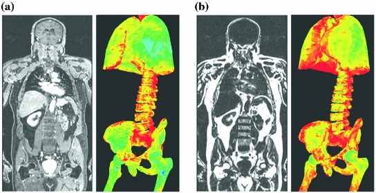
Fig. 3

Trained image features. a Water image from a single patient, Pat1, and the water feature quality in terms of simulated errors (see [11]) being trained on all patients. b Fat image from Pat1 and the fat feature quality being estimated from all patients. The color scale shows high quality features (green) to low quality features (red). As can be observed, water features are better around the lungs, femur, and pelvis. However, features around the vertebrae appear similar, and a simultaneous segmentation on both the water and fat image is expected to provide most reliable results

3 Experiments

3.1 Materials

Dixon MR images from 25 patients were acquired on a 3T MR Scanner (Philips Ingenuity TF PET/MR, Best, The Netherlands) using a quadrature body coil, with TR / TE $$_1$$