Voting for Robust Color Edge Detection

is given by:

$\begin{aligned} \mathrm {TV}({\mathbf {{{p}}}}) = \displaystyle \sum _{\mathbf {{{q}}}\in \mathcal {N}({\mathbf {{{p}}}})}\mathrm {SV}({\mathbf {{{v}}}}, \mathrm {S}_{{\mathbf {{{q}}}}}) + \mathrm {PV}({\mathbf {{{v}}}}, \mathrm {P}_{{\mathbf {{{q}}}}}) + \mathrm {BV}({\mathbf {{{v}}}}, \mathrm {B}_{{\mathbf {{{q}}}}}), \end{aligned}$

(1)

where ${\mathbf {{{q}}}}$ represents each of the points in the neighborhood of ${\mathbf {{{p}}}}, \,\mathcal {N}({\mathbf {{{p}}}}), \,\mathrm {SV}, \,\mathrm {PV}$ and $\mathrm {BV}$ are the stick, plate and ball tensor votes cast to ${\mathbf {{{p}}}}$ by every component of ${\mathbf {{{q}}}},\, {\mathbf {{{ v}}}}={\mathbf {{{p}}}}-{\mathbf {{{q}}}}$ , and $\mathrm {S}_{\mathbf {{{q}}}}, \,\mathrm {P}_{\mathbf {{{q}}}}$ and $\mathrm {B}_{\mathbf {{{q}}}}$ are the stick, plate and ball components of the tensor at $\mathbf {{{q}}}$ respectively. These components are given by:

$\begin{aligned} \mathrm {S}_{\mathbf {{{q}}}}&= (\lambda _1 -\lambda _2) \left( \mathbf {{{e}}_1{{e}}_1}^T\right) , \end{aligned}$

(2)

$\begin{aligned} \mathrm {P}_{\mathbf {{{q}}}}&= (\lambda _2-\lambda _3)\left( \mathbf {{{e}}_1{{e}}_1}^T+\mathbf {{{ e}}_2{{e}}_2} ^T\right) , \end{aligned}$

(3)

$\begin{aligned} \mathrm {B}_{\mathbf {{{q}}}}&= \lambda _3 \left( \mathbf {{{e}}_1{{e}}_1}^T+\mathbf {{{e}}_2{{e}}_2}^T+\mathbf {{{e}}_3{{e}}_3}^T\right) , \end{aligned}$

(4)

where $\lambda _i$ and $\mathbf {{{e}}_i}$ are the

th largest eigenvalue and its corresponding eigenvector of the tensor at $\mathbf {{{q}}}$ . Saliency measurements can be estimated from an analysis of the eigenvalues of the resulting tensors. Thus, $s_1=(\lambda _1 -\lambda _2),\, s_2=(\lambda _2 -\lambda _3)$ , and $s_3=\lambda _3$ can be used as measurements of surfaceness, curveness and junctionness respectively.

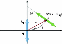
Fig. 1

Stick tensor voting. A stick $\mathrm {S}_{\mathbf {{q}}}$ casts a stick vote $\mathrm {SV}(\mathbf {{v}},\mathrm {S}_{\mathbf {{q}}})$ to $\mathbf {{p}}$ , which corresponds to the most likely tensorized normal at $\mathbf {{p}}$

A stick tensor is a tensor with only a single eigenvalue greater than zero. Stick tensors are processed through the so-called stick tensor voting. The process is illustrated in Fig. 1. Given a known stick tensor $\mathrm {S}_{\mathbf {{{q}}}}$ at $\mathbf {{{q}}}$ , the orientation of the vote cast by $\mathbf {{{q}}}$ to $\mathbf {{{p}}}$ can be estimated by tensorizing the normal of a a circumference at $\mathbf {{{p}}}$ that joins $\mathbf {{{q}}}$ and $\mathbf {{{p}}}$ . This vote is then weighted by a decaying scalar function,

. The stick tensor vote is given by [20]:

$\begin{aligned} \mathrm {SV}(\mathbf {{{v}}},\mathrm {S}_{\mathbf {{{q}}}}) = w_s\, R_{2\theta }~\mathrm {S}_{\mathbf {{{q}}}}~R_{2\theta }^T, \end{aligned}$

(5)

where $\theta$ is shown in Fig. 1 and $R_{2\theta }$ represents a rotation with respect to the axis $\mathbf {{{v}}} \times ( \mathrm {S}_{\mathbf {{{q}}}} ~ \mathbf {{{v}}} )$ , which is perpendicular to the plane that contains $\mathbf {{{v}}}$ and $\mathrm {S}_{\mathbf {{{q}}}}$ ; and

is an exponential decaying function that penalizes the arc-length

, and the curvature of the circumference, $\kappa$ :

$\begin{aligned} w_s = \left\{ \begin{array}{ll} e^{-\frac{l^2}{\sigma ^2} +b\kappa ^2}&{} {\text {if}}\;\theta \le \pi /4\\ 0 &{} {\text {otherwise}},\end{array}\right. \end{aligned}$

(6)

where $\sigma$ and

are parameters to weight the scale and the curvature respectively.

In turn, a plate tensor is a tensor with $\lambda _1=\lambda _2\ge 0$ and $\lambda _3=0$ . Plate tensors are processed through the so-called plate tensor voting. The plate tensor voting uses the fact that any plate tensor $\mathrm {P}$ , can be decomposed into all possible stick tensors inside the plate. Let $\mathrm {S}_\mathrm {P}(\beta )=R_{\beta }\mathbf {{{e}}_1{{e}}_1}^TR_{\beta }^T$ be a stick inside the plate $\mathrm {P}$ , with $\mathbf {{{e}}_1}$ being its principal eigenvector, and $R_{\beta }$ being a rotation with respect to an axis perpendicular to $\mathbf {{{e}}_1}$ and $\mathbf {{{e}}_2}$ . Thus, the plate vote is defined as [20]:

$\begin{aligned} \mathrm {PV}(\mathbf {{{v}}},\mathrm {P}_{\mathbf {{{q}}}}) = \frac{\lambda _{1_{\mathrm {P}_{\mathbf {{{q}}}}}}}{\pi } \int _0^{2\pi } \mathrm {SV}(\mathbf {{{v}}},\mathrm {S}_{\mathrm {P}_{\mathbf {{{q}}}}}(\beta )) ~d\beta , \end{aligned}$

(7)

where $\lambda _{1_{\mathrm {P}_{\mathbf {{{q}}}}}}$ is the largest eigenvalue of $\mathrm {P}_{\mathbf {{{q}}}}$ .

Finally, a ball tensor is a tensor with $\lambda _1=\lambda _2=\lambda _3\ge 0$ . The ball tensor voting is defined in a similar way as the plate tensor voting. Let $\mathrm {S}_{\mathrm {B}}(\phi , \psi )$ be a unitary stick tensor oriented in the direction $(1,\phi ,\psi )$ in spherical coordinates. Then, any ball tensor $\mathrm {B}$ can be written as [20]:

$\begin{aligned} \mathrm {BV}({\mathbf {{{v}}},\mathrm {B}_{\mathbf {{{q}}}}}) = \frac{3\lambda _{1_{\mathrm {B}_{\mathbf {{q}}}}}}{4\pi } \int _\varGamma \mathrm {SV}(\mathbf {{{v}}},\mathrm {S}_{\mathrm {B}_{\mathbf {{{q}}}}}(\phi , \psi )) ~d\varGamma , \end{aligned}$

(8)

where $\varGamma$ represents the surface of the unitary sphere, and $\lambda _{1_{\mathrm {B}_{\mathbf {{{q}}}}}}$ is the largest eigenvalue of $\mathrm {B}_{\mathbf {{{q}}}}$ .

2.2 Color Edge Detection Through the Classical Tensor Voting

In Ref. [21], we showed that the classical tensor voting and the well-known structure tensor [8] are closely related. These similarities were used in [21] to extend classical tensor voting to different types of images, especially color images. This extension can be used to extract edges. This subsection summarizes that method for gray-scale and color images.

2.2.1 Gray-Scale Images

Tensor voting can be adapted in order to robustly detect edges in gray-scale images by following three steps. First, the tensorized gradient, $\nabla u\nabla u^T$ , is used to initialize a tensor at every pixel. Second, the stick tensor voting is applied in order to propagate the information encoded in the tensors. In this case, it is not necessary to apply the plate and ball voting processes since the plate and ball components are zero at every pixel. Thus, tensor voting is reduced to:

$\begin{aligned} \mathrm {TV}(\mathbf {{{p}}}) = \displaystyle \sum _{\mathbf {{{q}}}\in \mathcal {N}(\mathbf {{{p}}})}\mathrm {SV}(\mathbf {{{v}}},\nabla u_{\mathbf {{{q}}}}\nabla u_{\mathbf {{{q}}}}^T). \end{aligned}$

(9)

Finally, the resulting tensors are rescaled by the factor:

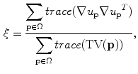
$\begin{aligned} \xi = \frac{\displaystyle \sum _{\mathbf {{{p}}} \in \Omega } trace(\nabla u_{\mathbf {{{p}}}} {\nabla u_{\mathbf {{{p}}}}}^T)}{\displaystyle \sum _{\mathbf {{{p}}} \in \Omega } trace(\mathrm {TV}(\mathbf {{{p}}}))}, \end{aligned}$

(10)

in order to renormalize the total energy of the tensorized gradient, where $\Omega$ refers to the given image.

After having applied tensor voting and the energy normalization step, the principal eigenvalue $\lambda _1$ of the resulting tensors can be used to detect edges, since it attains high values not only at boundaries but also at corners.

2.2.2 Color Images

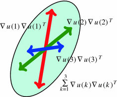
Figure 2 shows the two possible options to extend tensor voting to color images using the adaptation proposed in the previous subsection. The first option is to apply the stick tensor voting independently to every channel and then adding the individual results, that is:

$\begin{aligned} \mathrm {TV}(\mathbf {{{p}}}) = \displaystyle \sum _{k=1}^{3}\sum _{\mathbf {{{q}}}\in \mathcal {N}(\mathbf {{{p}}})}\alpha _k~\mathrm {SV}(\mathbf {{{v}}},\nabla u_{\mathbf {{{q}}}}(k)\nabla u_{\mathbf {\text {{q}}}}(k)^T), \end{aligned}$

(11)

where $\nabla u(k)$ is the gradient at color channel $$k$$

, and $\alpha _k$ are weights used to give different relevance to every channel.

Fig. 2

Tensor voting can be applied to the color channels independently (the red, green and blue sticks) or to the sum of the tensorized gradients (the ellipse)

The second option is to apply (1) to the sum of tensorized gradients, with $\mathrm {S}_{\mathbf {{{q}}}},\, \mathrm {P}_{\mathbf {{{q}}}}$ and $\mathrm {B}_{\mathbf {{{q}}}}$ being the stick, plate and ball components of $\mathrm {T}_{\mathbf {{{q}}}}=\sum _{k=1}^{3} \alpha _k \nabla u_{\mathbf {{{q}}}}(k) {\nabla u_{\mathbf {{{q}}}}(k)}^T$ . For two-dimensional images, the computation of plate votes can be avoided since $\mathrm {P}_{\mathbf {{{q}}}}=0$ . Thus, the first option has the advantage that only the application of stick tensor voting is necessary, whereas the second option requires stick and ball tensor voting.

In practice, both strategies are very similar since $\mathrm {T}_{\mathbf {{q}}}\approx \mathrm {S}_{\mathbf {{q}}}$ in most pixels of images of natural scenes [21]. Thus, in the experiments of Section 5, the first option has been used for the majority of pixels, whereas the second one only in those pixels in which the aforementioned approximation is not valid. In practice, the first option can be applied when the angle between any pair of gradients is below a threshold.

Similarly to the case of gray-scale images, the classical tensor voting can be used to detect edges by means of the principal eigenvalue $\lambda _1$ of the resulting tensor, after an energy normalization step similar to the one of (10).

Since this method does not apply any pre-processing step, its robustness must completely rely on the robustness of the classical tensor voting. This could not be sufficient in highly noisy scenarios. Thus, in order to improve the results it is necessary to iterate the method. By iterating tensor voting, the most significant edges can be reinforced at the expense of discarding small ridges. According to our experiments, a few iterations (two or three) usually give good results for both noisy and noiseless images.

3 Color Edge Detection Through an Adapted Tensor Voting

It is important to remark that tensor voting is a methodology in which information encoded through tensors is propagated and aggregated in a local neighborhood. Thus, it is possible to devise more appropriate methods for specific applications by tailoring the way in which tensors are encoded, propagated and aggregated, while maintaining the tensor voting spirit. In this line, we introduced a method for image denoising [17, 19] that can also be applied to robust color edge detection, since both problems can be tackled at the same time [18]. The next subsections detail the edge detector.

3.1 Encoding of Color Information

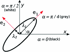
Before applying the proposed method, color is converted to the CIELAB space. Every CIELAB channel is then normalized to the range $\left[ 0,\pi /2\right]$ . In the first step of the method, the information of every pixel is encoded through three second-order 2D tensors, one for each normalized CIELAB color channel.

Three perceptual measures are encoded in the tensors associated with every input pixel, namely: the normalized color at the pixel (in the specific channel), a measure of local uniformity (how edgeless its neighborhood is), and an estimation of edginess. Figure 3 shows the graphical interpretation of a tensor for channel $$L$$

. The normalized color is encoded by the angle $\alpha$ between the $$x$$

axis, which represents the lowest possible color value in the corresponding channel, and the eigenvector corresponding to the largest eigenvalue. For example, in channel $$L$$

, a tensor with $\alpha = 0$ encodes black, whereas a tensor with $\alpha = \dfrac{\pi }{2}$ encodes white. In addition, local uniformity and edginess are encoded by means of the normalized $\hat{s_{1}} = (\lambda _1 - \lambda _2) / \lambda _1$ and $\hat{s_{2}} = \lambda _2 / \lambda _1$ saliencies respectively. Thus, a pixel located at a completely uniform region is represented by means of three stick tensors, one for each color channel. In contrast, a pixel located at an ideal edge is represented by means of three ball tensors, one for every color channel.

Fig. 3

Encoding process for channel $$L$$

. Color, uniformity and edginess are encoded by means of $\alpha$ and the normalized saliencies $\hat{s_{1}}=(\lambda _1-\lambda _2 ) / \lambda _1$ and $\hat{s_{2}}=\lambda _2/\lambda _1$ respectively

Before applying the voting process, it is necessary to initialize the tensors associated with every pixel. The colors of the noisy image can be easily encoded by means of the angle $\alpha$ between the $$x$$

axis and the principal eigenvector, as described above. However, since metrics of uniformity and edginess are usually unavailable at the beginning of the voting process, normalized saliency $\hat{s_{1}}$ is initialized to one and normalized saliency $\hat{s_{2}}$ to zero. These initializations allow the method to estimate more appropriate values of the normalized saliencies for the next stages, as described in the next subsection. Thus, the initial color information of a pixel is encoded through three stick tensors oriented along the directions that represent that color in the normalized CIELAB channels:

$\begin{aligned} \mathrm {T}_k(\mathbf {p})= \mathbf {t}_k(\mathbf {p})~ \mathbf {t}_k(\mathbf {p})^T, \end{aligned}$

(12)

where $\mathrm {T}_k(\mathbf {p})$ is the tensor of the $$k$$

th color channel ( $L,\, a$ and $$b$$

) at pixel $\mathbf {p},\, \mathbf {{t}}_k(\mathbf {{p}})=\left[ \cos \left( \mathrm {C}_k(\mathbf {{p}})\right) ~~ \sin \left( \mathrm {C}_k(\mathbf {{p}})\right) \right] ^T$ , and $\mathrm {C}_k(\mathbf {{p}})$ is the normalized value of the $$k$$

-th color channel at $\mathbf {{p}}$ .

3.2 Voting Process

The voting process requires three measurements for every pair of pixels $\mathbf {{p}}$ and $\mathbf {{q}}$ : the perceptual color difference, $\Delta E_{\mathbf {{p}}\mathbf {{q}}}$ ; the joint uniformity measurement, $U_k(\mathbf {{p}},\mathbf {{q}})$ , used to determine if both pixels belong to the same region; and the likelihood of a pixel being impulse noise, $\eta _k(\mathbf {{p}})$ . $\Delta E_{\mathbf {{p}}\mathbf {{q}}}$ is calculated through CIEDE2000 [13], while

$\begin{aligned} U_k({\mathbf {{p}}},{\mathbf {{q}}}) = \hat{s_{1k}}({\mathbf {p}}) ~\hat{s}_{1k}(\mathbf {{q}}), \end{aligned}$

(13)

and

$\begin{aligned} \eta _k(\mathbf {{p}})=\left\{ \begin{array}{ll} \hat{s_{2c}}(\mathbf {{p}}) - \mu _{\hat{s_{2c}}}(\mathbf {{p}}) &{}~~ \text {if}\, \mathbf {{p}} \,\text {is located at a local maximum}\\ 0 &{} ~~\text {otherwise} \end{array}\right. , \end{aligned}$

(14)

where $\mu _{\hat{s_{2c}}}(\mathbf {{p}})$ represents the mean of $\hat{s_{2c}}$ over the neighborhood of $\mathbf {{p}}$ .

In the second step of the method, the tensors associated with every pixel are propagated to their neighbors through a convolution-like process. This step is independently applied to the tensors of every channel ( $L,\, a$ and $$b$$

). The voting process is carried out by means of specially designed tensorial functions referred to as propagation functions, which take into account not only the information encoded in the tensors but also the local relations between neighbors. Two propagation functions are proposed for edge detection: a stick and a ball propagation function. The stick propagation function is used to propagate the most likely noiseless color of a pixel, while the ball propagation function is used to increase edginess where required. The application of the first function leads to stick votes, while the application of the second function produces ball votes. Stick votes are used to eliminate noise and increase the edginess where the color of the voter and the voted pixels are different. Ball votes are used to increase the relevance of the most important edges.

A stick vote can be seen as a stick-shaped tensor, $\mathrm {ST}_k(\mathbf {{p}})$ , with a strength modulated by three scalar factors. The proposed stick propagation function, $\mathrm {S}_k(\mathbf {{p}},\mathbf {{q}})$ , which allows a pixel $\mathbf {{p}}$ to cast a stick vote to a neighboring pixel $\mathbf {{q}}$ for channel $$k$$

is given by:

$\begin{aligned} \mathrm {S}_k(\mathbf {{p}},\mathbf {{q}}) = GS(\mathbf {{p}},\mathbf {{q}}) ~\overline{\eta _k}(\mathbf {{p}}) ~{SV}^{\prime }_k(\mathbf {{p}},\mathbf {{q}}) ~ \mathrm {ST}_k(\mathbf {{p}}), \end{aligned}$

(15)

with $\mathrm {ST}_k(\mathbf {{p}}),\, GS(\mathbf {{p}},\mathbf {{q}}), \overline{\eta _k}(\mathbf {{p}})$ and ${SV}^{\prime }_k(\mathbf {{p}},\mathbf {{q}})$ being defined as follows. First, the tensor $\mathrm {ST}_k(\mathbf {{p}})$ encodes the most likely normalized noiseless color at $\mathbf {{p}}$ . Thus, $\mathrm {ST}_k(\mathbf {{p}})$ is defined as the tensorized eigenvector corresponding to the largest eigenvalue of the voter pixel, that is:

$\begin{aligned} \mathrm {ST}_k(\mathbf {{p}}) = \mathbf {{e}}_{1k}(\mathbf {{p}})~\mathbf {{e}}_{1k}(\mathbf {{p}})^T, \end{aligned}$