Weighted Principal Component Regression for High-Dimensional Prediction

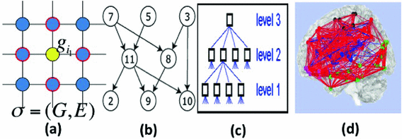
by using high-dimensional data $\mathbf{x}=\{\mathbf{x}_{g}: g\in \mathcal G\}$ measured on a graph $\zeta =({\mathcal G}, {\mathcal E})$ , where ${\mathcal E}$ is the edge set of $\zeta$ and $\mathcal G=\{ g_1, \ldots , g_m\}$ is a set of vertexes, in which m is the total number of vertexes in ${\mathcal G}.$ The response $\mathbf{Y}$ may include cognitive outcome, disease status, and the early onset of disease, among others. Standard graphs including both directed and undirected graphs have been widely used to build complex patterns [10]. Examples of graphs are linear graphs, tree graphs, triangulated graphs, and 2-dimensional (2D) (or 3-dimensional (3D)) lattices, among many others (Fig. 1). Examples of $\mathbf{x}$ on the graph $\zeta =({\mathcal G}, {\mathcal E})$ include time series and genetic data measured on linear graphs and imaging data measured on triangulated graphs (or lattices). Particularly, various structural and functional neuroimaging data are frequently measured in a 3D lattice for the understanding of brain structure and function and their association with neuropsychiatric and neurodegenerative disorders [9].

Fig. 1.

Illustration of graph data structure $\zeta =({\mathcal G}, {\mathcal E})$ : (a) two-dimensional lattice; (b) acyclic directed graph; (c) tree; (d) undirected graph.

The aim of this paper is to develop a new framework of spatially weighted principal component regression (SWPCR) to use $\mathbf{x}$ on graph $\zeta =\{\mathcal G, \mathcal E\}$ to predict $\mathbf{Y}$ . Four major challenges arising from such development include ultra-high dimensionality, low sample size, spatially correlation, and spatial smoothness. SWPCR is developed to address these four challenges when high-dimensional data on graphs $\zeta$ share two important features including spatial smoothness and intrinsically low dimensional structure. Compared with the existing literature, we make several major contributions as follows:

(i) SWPCR is designed to efficiently capture the two important features by using some recent advances in smoothing methods, dimensional reduction methods, and sparse methods.
(ii) SWPCR provides a powerful dimension reduction framework for integrating feature selection, smoothing, and feature extraction.
(iii) SWPCR significantly outperforms the competing methods by simulation studies and the real data analysis.

2 Spatially Weighted Principal Component Regression

In this section, we first describe the graph data that are considered in this paper. We formally describe the general framework of SWPCR.

2.1 Graph Data

Consider data from n independent subjects. For each subject, we observe a $q \times 1$ vector of discrete or continuous responses, denoted by $\mathbf{y}_i=(\mathbf{y}_{i, 1}, \ldots ,\mathbf{y}_{i, q})^T$ , and a $m\times 1$ vector of high dimensional data $\mathbf{x}_i=\{\mathbf{x}_{i, g}: g\in \mathcal G\}$ for $i=1, \ldots , n$ . In many cases, q is relatively small compared with n, whereas m is much larger than n. For instance, in many neuroimaging studies, it is common to use ultra-high dimensional imaging data to classify a binary class variable. In this case, $$q=1$$

, whereas m can be several million number of features. In many applications, $\mathcal G=\{ g_1, \ldots , g_{m}\}$ is a set of prefixed vertexes, such as voxels in 2D or 3D lattices, whereas the edge set ${\mathcal E}$ may be either prefixed or determined by $\mathbf{x}_i$ (or other data).

2.2 SWPCR

We introduce a three-stage algorithm for SWPCR to use high-dimensional data $\mathbf{x}$ to predict a set of response variables $\mathbf{Y}$ . The key stages of SWPCR can be described as follows.

Stage 1. Build an importance score vector (or function) $W_I: \mathcal G\rightarrow R^+$ and the spatial weight matrix (or function) $W_E: \mathcal G\times \mathcal G\rightarrow R$ .
Stage 2. Build a sequence of scale vectors $\{\mathbf{s}_0=(\mathbf{s}_{E,0}, \mathbf{s}_{I, 0}), \cdots , \mathbf{s}_L=(\mathbf{s}_{E,L}, \mathbf{s}_{I, L})\}$ ranging from the smallest scale vector $\mathbf{s}_0$ to the largest scale vector $\mathbf{s}_L$ . At each scale vector $\mathbf{s}_\ell$ , use generalized principal component analysis (GPCA) to compute the first few principal components of an $n \times m$ matrix $X = (\mathbf x_1 \cdots \mathbf x_n)^T$ , denoted by ${A}(\mathbf{s}_\ell )$ , based on $W_E(\cdot , \cdot )$ and $W_I(\cdot )$ for $\ell =0, \ldots , L$ .
Stage 3. Select the optimal $0\le \ell ^* \le L$ and build a prediction model (e.g., high-dimensional linear model) based on the extracted principal components ${A}(\mathbf{s}_{\ell ^*})$ and the responses $\mathbf{Y}$ .

We slightly elaborate on these stages. In Stage 1, the important scores $w_{I, g}$ play an important feature screening role in SWPCR. Examples of $w_{I, g}=W_I(g)$ in the literature can be generated based on some statistics (e.g., Pearson correlation or distance correlation) between $\mathbf{x}_g$ and $\mathbf{Y}$ at each vertex g. For instance, let p(g) be the Pearson correlation at each vertex g and then define

$\begin{aligned} w_{I,g}=- m \; \mathrm{log} ({p(g)})/\left[ -\sum _{g \in \mathcal G}\mathrm{log} ({p(g)})\right] . \end{aligned}$

(1)

In Stage 1, without loss of generality, we focus on the symmetric matrix $W_E=(w_{E, gg'})\in R^{p\times p }$ throughout the paper. The element $w_{E, gg'}$ is usually calculated by using various similarity criteria, such as Gaussian similarity from Euclidean distance, local neighborhood relationship, correlation, and prior information obtained from other data [21]. In Sect. 2.3, we will discuss how to determine $$W_E$$

and

while explicitly accounting for the complex spatial structure among different vertexes.

In Stage 2, at each scale vector $\mathbf{s}_\ell =(\mathbf{s}_{E, \ell },\mathbf{s}_{I, \ell })$ , we construct two matrices, denoted by $Q_{E, \ell }$ and $Q_{I, \ell }$ based on $$W_E$$

and

as follows:

$\begin{aligned} Q_{E, \ell }=F_1(W_E, \mathbf{s}_{E, \ell })~~\text{ and }~~ Q_{I, \ell }=\text{ diag }(F_2(W_I, s_{I, \ell })), \end{aligned}$

(2)

where $F_1: R^{p\times p}\times R^+\rightarrow R^{p\times p}$ and $F_2: R^p\times R^+\rightarrow R^p$ are two known functions. For instance, let $\mathbf{1}(\cdot )$ be an indicator function, we may set

$\begin{aligned} F_2(W_I, s_{I, \ell })=\left( \mathbf{1}(w_{I, g_1}\ge s_{I, \ell }), \cdots , \mathbf{1}(w_{I, g_{m}}\ge s_{I, \ell })\right) ^T, \end{aligned}$

(3)

to extract ’significant’ vertexes. There are various ways of constructing $Q_{E, \ell }$ . For instance, one may set $Q_{E, \ell }$ as

$\begin{aligned} Q_{E, \ell }=\left( |w_{E, gg'}|\mathbf{1}(|w_{E, gg'}|\ge s_{E, \ell ; 1}, D(g, g')\le s_{E, \ell ; 2})\right) , \end{aligned}$

where $\mathbf{s}_{E, \ell }=(s_{E, \ell ; 1}, s_{E, \ell ; 2})^T$ and $$D(g, g')$$

is a graph-based distance between vertexes g and $$g'$$

. The value of $s_{E, \ell ; 2}$ controls the number of vertexes in $\{ g' \in \mathcal G: D(g, g')\le s_{E, \ell ; 2}\}$ , which is a patch set at vertex g [18], whereas $s_{E, \ell ; 1}$ is used to shrink small $|w_{E, gg'}|$ s into zero.

After determining $Q_{E, \ell }$ and $Q_{I, \ell }$ , we set $\varSigma _c= Q_{E, \ell } Q_{I, \ell } Q_{I, \ell }^T Q_{E, \ell }^T$ and $\varSigma _r=I_n$ for independent subjects. Let $\widetilde{\mathbf{X}}$ be the centered matrix of $\mathbf X$ . Then we can extract K principal components through minimize the following objective function given by

$\begin{aligned} ||\widetilde{\mathbf{X}}-U D V ^T||^2 ~~\text{ subject } \text{ to }~~ U^T\varSigma _r U= V ^T \varSigma _c V ={I}_K ~~\text{ and }~~ \text{ diag }( D )\ge 0. \end{aligned}$

(4)

If we consider correlated observations from multiple subjects, we may use $\varSigma _r$ to explicitly model their correlation structure. The solution $(U_\ell , D _\ell , V_\ell )$ of the objective function (4) at $\mathbf{s}_\ell$ is the SVD of $\widetilde{\mathbf{X}}_{R, \ell }=\widetilde{\mathbf{X}} Q_{E, \ell } Q_{I, \ell }$ . The we can use a GPCA algorithm to simultaneously calculate all components of $(U_\ell , D _\ell , V_\ell )$ for a fixed K as follows. In practice, a simple criterion for determining K is to include all components up to some arbitrary proportion of the total variance, say 85 $\%$ .

For ultra-high dimensional data, we consider a regularized GPCA to generate $(U_\ell , D _\ell , V_\ell )$ by minimizing the following objective function

$\begin{aligned} ||\widetilde{\mathbf{X}}_{R, \ell }-\sum _{k=1}^K d_{k, \ell }\mathbf{u}_{k, \ell } \mathbf{v}_{k, \ell }^T||^2+\lambda _\mathbf{u}\sum _{k=1}^K P_1(d_{k, \ell }\mathbf{u}_{k, \ell })+\lambda _\mathbf{v}\sum _{k=1}^KP_2(d_{k, \ell }\mathbf{v}_{k, \ell })~ \end{aligned}$

(5)

subject to $\mathbf{u}_{k, \ell }^T\mathbf{u}_{k, \ell }\le 1$ and $\mathbf{v}_{k, \ell }^T\mathbf{v}_{k, \ell }\le 1$ for all k, where $\mathbf{u}_{k, \ell }$ and $\mathbf{v}_{k, \ell }$ are respectively the k-th column of $U_\ell$ and $V_\ell$ . We use adaptive Lasso penalties for $P_1(\cdot )$ and $P_2(\cdot )$ and then iteratively solve (5) [1]. For each $$k_0$$

, we define $\mathbf{E}_{\ell , k_0}=\widetilde{\mathbf{X}}_{R, \ell }-\sum _{k\not =k_0}d_{k, \ell }\mathbf{u}_{k, \ell } \mathbf{v}_{k, \ell }^T$ and minimize

$\begin{aligned} ||\mathbf{E}_{\ell , k_0}-d_{k_0, \ell }\mathbf{u}_{k_0, \ell } \mathbf{v}_{k_0, \ell }^T||^2+\lambda _\mathbf{u} P_1(d_{k_0, \ell }\mathbf{u}_{k_0, \ell })+\lambda _\mathbf{v}P_2(d_{k_0, \ell }\mathbf{v}_{k_0, \ell })~ \end{aligned}$

(6)

subject to $\mathbf{u}_{k_0, \ell }^T\mathbf{u}_{k_0, \ell }\le 1$ and $\mathbf{v}_{k_0, \ell }^T\mathbf{v}_{k_0, \ell }\le 1$ . By using the sparse method in [12], we can calculate the solution of (6), denoted by $(\hat{d}_{k_0, \ell }, \hat{\mathbf{u}}_{k_0, \ell }, \hat{\mathbf{v}}_{k_0, \ell })$ . In this way, we can sequentially compute $(\hat{d}_{k, \ell }, \hat{\mathbf{u}}_{k, \ell }, \hat{\mathbf{v}}_{k, \ell })$ for $k=1, \ldots , K$ .

In Stage 3, select $\ell ^*$ as the minimum point of the objective function (5) or (6) . let $Q_{F,\ell ^*}= Q_{E, \ell ^*} Q_{I, \ell ^*} V_{\ell ^*} D _{\ell ^*}^{-1}$ and then K principal components ${A}(\mathbf{s}_{\ell ^*}) =\mathbf{X} Q_{F,\ell ^*}$ . Moreover, K is usually much smaller than $\min (n, m)$ . Then, we build a regression model with $\mathbf{y}_i$ as responses and ${A}_i$ (the i-th row of ${A}(\mathbf{s}_{\ell ^*})$ ) as covariates, denoted by $R(\mathbf{y}_i, {A}_i; \mathbf {\theta })$ , where $\mathbf {\theta }$ is a vector of unknown (finite-dimensional or nonparametric) parameters. Specifically, based on $\{(\mathbf{y}_i, {A}_i)\}_{i\ge 1}$ , we use an estimation method to estimate $\mathbf {\theta }$ as follows:

$\begin{aligned} \widehat{\mathbf {\theta }}=\text{ argmin }_{\mathbf {\theta }}\{\rho \left( R, \mathbf {\theta }, \{(\mathbf{y}_i, {A}_i)\}_{i\ge 1}\right) +\lambda P_3(\mathbf {\theta })\}, \end{aligned}$

where $\rho (\cdot , \cdot , \cdot )$ is a loss function, which depends on both the regression model and the data, and $P_3(\cdot )$ is a penalty function, such as Lasso. This leads to a prediction model $R(\mathbf{y}_i, {A}_i; \mathbf {\theta })$ . For instance, for binary response $\mathbf{y}_i=1$ or 0, we may consider a sparse logistic model given by $\text{ logit }(P(\mathbf{y}_i=1| A_i))= A_i^T\mathbf {\theta }$ for $R(\mathbf{y}_i, {A}_i; \mathbf {\theta })$ .