Computed Tomography

A. X-ray tubes

–High-frequency power supplies are used in computed tomography (CT), capable of providing stable tube currents and voltages.

–Modern CT scanners make use of slip ring technology in which high voltage is supplied to the tube through contact rings in the gantry.

–Tube voltages range from 80 to 140 kV.

–Tube currents can range up to 1,000 mA.

–Tube currents are frequently modulated as the x-ray tube rotates around the patient.

–Tube currents increase when the path length increases, as in a lateral abdominal projection compared to an anteroposterior (AP) projection.

–Time for a 360-degree rotation of the x-ray tube currently ranges between 0.3 and 2 seconds.

–Table 5.1 shows how x-ray tube rotation times have been reduced since the introduction of CT scanners into clinical practice in the early 1970s.

–Tube current of 800 mA and rotation time of 0.3 s corresponds to 240 mAs.

–Power loading on CT x-ray tubes can be as high as ~100 kW.

–A tube voltage of 120 kV and tube current of 830 mA corresponds to 100 kW.

–Table 5.1 shows how x-ray tube power capabilities have increased since the early 1970s.

–CT x-ray tubes have a large focal spot with a size of ~1 mm, which can tolerate a power loading of 100 kW.

–Small x-ray tube focal spots are about half the size of the large focal spot and can tolerate no more than ~25 kW.

–Heat loading on CT x-ray tubes is generally high, requiring high anode heat capacities.

–X-ray tube anode heat capacities are high, and can exceed 4 MJ.

–Anode heat dissipation rates are ~10 kW.

–Recent innovations in x-ray tube design include a rotating envelope vacuum vessel (Straton tube).

–The Straton tube is relatively light and has very high heat dissipation rate that is >60 kW.

–CT x-ray tubes are very expensive, with the price of some tubes exceeding $200,000.

B. Filtration

–The x-ray tube anode–cathode axis is positioned perpendicular to the imaging plane to reduce the heel effect.

–Copper or aluminum filters are used to filter the x-ray beam.

–The typical filtration on a CT x-ray tube is ~6 mm Al.

–The heavy filtration used with CT scanners typically produces a beam with an aluminum half-value layer (HVL) of up to 10 mm Al.

–Heavy x-ray beam filtering reduces x-ray beam hardening effects.

–A bow tie filter is used to minimize the dynamic range of exposures at the detector.

–Bow tie filters attenuate little in the center, but attenuation increases with increasing distance from the central ray.

TABLE 5.1 Representative Values of X-ray Tube Power and Minimum Scan Times in CT Scanning

–Bow tie filters are made of a low Z material such as Teflon to minimize beam hardening differences.

–Bow tie filters also reduce scatter and patient dose.

C. Collimation

–Collimators are located at the x-ray tube as well as at the x-ray detectors.

–Collimation defines the section thickness on a single-slice scanner.

–Collimation defines the total beam width in multidetector CT (MDCT) systems.

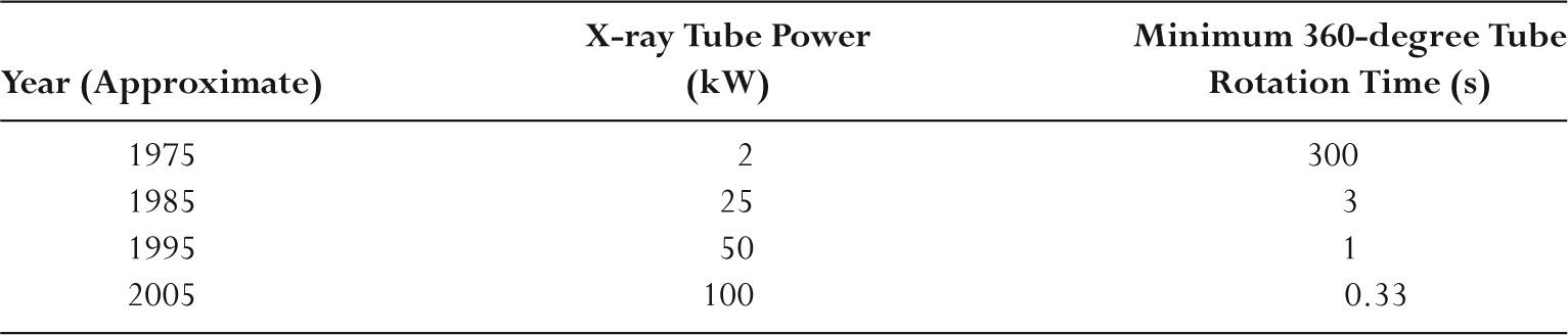
–The beam width on a 64-slice CT scanner is ~40 mm.

–The beam width on a 320-slice scanner is ~160 mm.

–Collimators also help reduce the amount of scatter radiation reaching the CT detectors.

–Some scanners have (optional) antiscatter collimation in the form of thin lamellae (e.g., 100-μm tantalum sheets).

–Antiscatter collimation is located between the detector elements oriented along the long patient axis and aligned with the x-ray focus.

–Some CT scanners use a high-resolution comb whose teeth serve to reduce the detector aperture width.

–Use of a high-resolution comb improves resolution but will also reduce dose efficiencies.

D. Radiation detectors

–Each detector measures the intensity of radiation transmitted through the patient along one ray.

–Detectors are separated from each other by a dead space of ~0.1 mm, which reduces the geometric efficiency.

–Geometric efficiencies are ~90% for detectors that are 1 mm wide.

–Modern CT scanners use scintillators that produce light when x-ray photons are absorbed.

–Scintillation detectors are coupled to a light detector.

–Common light detectors are photomultiplier tubes and photodiodes.

–CT detectors should have a good temporal response and rapid signal decay.

–CT detectors should also have low afterglow characteristics.

–Detectors have high quantum efficiency, which is the percentage of incident x-ray photons that are absorbed.

–CT detectors have a quantum efficiency of >90%.

–Scintillators convert ~10% of the absorbed x-ray energy into light energy (conversion efficiency).

–In CT detectors, an electric signal is produced that is proportional to the incident radiation intensity.

–The signal acquired by each detector is digitized and stored in a computer.

–The most common material used in solid-state detectors is cadmium tungstate (CdWO₄), which is an efficient x-ray detector.

–Cesium iodide, calcium fluoride, and bismuth germanate may also be used.

E. Detector arrays

–Single-slice CT scanners had a single detector array.

–A detector array contains ~800 individual detectors in axial plane for each slice that is acquired.

–A single-slice CT scanner generates one tomographic image (slice) for each 360-degree rotation of the x-ray tube.

–Single-slice CT scanners are rapidly being replaced by multidetector CT (MDCT) scanners.

–MDCT scanners have a number of detector arrays that allow multiple tomographic images to be acquired per 360-degree rotation of the x-ray tube.

–Four-slice MDCT were introduced into clinical practice in 1998, which produce four images (slices) per 360-degree x-ray tube rotation.

–By 2004, 64-slice MDCT were in clinical operation.

–A 64-slice MDCT has 64 detector arrays, each with a dimension of ~0.6 along the long patient axis, which can generate 64 × 0.6 thick slices for each x-ray tube rotation.

–The beam width for this 64 slice CT scanner is ~40 mm (i.e., 64 × 0.6 mm).

–Figure 5.1 shows a schematic depiction of a 64-slice CT scanner.

–MDCT scanners have been developed to acquire 320 slices in one 360-degree rotation of the x-ray tube, with each slice having a thickness of 0.5 mm.

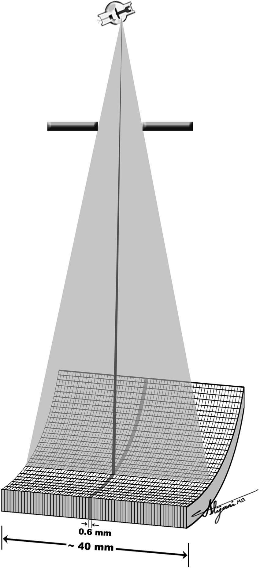
FIGURE 5.1 Schematic depiction of a MDCT with 64 rows of detector aligned along the long patient axis.

–A 320-slice CT scanner has a beam width of 160 mm (i.e., 320 × 0.5 mm) and covers the brain or left ventricle in one x-ray tube rotation.

–MDCT scanners with thin patient axis slices now have isotropic resolution.

–Isotropic resolution permits nonaxial reconstructions without stretching pixels.

II. IMAGES

A. Image acquisition

–For each position of the x-ray tube, a fan beam is passed through the patient.

–In body imaging, the fan beam angle is ~50 degrees.

–A fan beam of 50 degrees corresponds to a field of view with a 50-cm diameter.

–Measurements of the transmitted x-ray beam intensities are made by an array of detectors.

–The total x-ray transmission measured by each detector is the result of the sum of the attenuation by all the tissues the beam has passed through (i.e., ray sum).

–The collection of ray sums for all the detectors at a given tube position is called a projection.

–Each projection has ~800 individual data points corresponding to the ~800 individual detectors in a single array (single-slice scanner).

–Figure 5.2 shows the acquisition of a single projection at one position of the x-ray tube.

–Projection data sets are acquired at different angles around the patient.

–A CT image generally requires ~1,000 projections for a single rotation of the x-ray tube.

–A graphic plot of projections as a function of x-ray tube angle is called a sinogram.

–Figure 5.3 shows a typical sinogram that consists of projections acquired through all the angular positions of the x-ray tube as it rotates 360 degrees around the patient.

–CT images are derived by mathematical analysis of projection data sets (sinograms) at each location along the long patient axis.

B. Image reconstruction

–Generating an image from the acquired data involves determining the linear attenuation coefficients of the individual pixels in the image matrix.

–A mathematical algorithm takes the multiple projection data (raw data) and reconstructs the cross-sectional CT image (image data).

FIGURE 5.2 Schematic depiction of a single projection transmitted through the patient, consisting of ~700 individual rays.

FIGURE 5.3 Three projections as acquired at x-ray tube angles of 0 degrees, 90 degrees, and 180 degrees (left), and the resultant sinogram (right) showing all projections stacked on top of each other.

–Back projection allocates the measured total attenuation (ray sum) equally to each pixel along the x-ray path through the patient.

–Modern scanners use filtered back projection image reconstruction algorithms.

–Projection data are convolved with a (mathematical) filter before being back projected.

–Convolution is a type of mathematical multiplication.

–Image reconstruction involving millions of data points may be performed in less than a second using array processors (number crunchers).

–Different filters may be used in filtered back projection reconstruction.

–Commercial CT scanners typically offer six or seven filters for clinical use.

–The choice of filter in the reconstruction algorithm offers tradeoffs between spatial resolution and random noise.

–Some filters (e.g., bone) permit reconstruction of fine detail but with increased noise. Other filters (e.g., soft tissue) decrease noise but also decrease resolution.

–Table 5.2 shows how the amount of noise in reconstructed CT images varies with the type of reconstruction filter.

–The choice of the best filter to use with the reconstruction algorithm depends on the clinical task.

–Iterative (trial and error) methods such as algebraic reconstruction techniques (ART) have been used for image reconstruction.

–There is a resurgence of interest in iterative reconstruction techniques in CT.

–Iterative reconstruction algorithms may offer an effective means for minimizing CT artifacts (e.g., streak).

TABLE 5.2 Relative Image Noise Values as a Function of the Choice of CT Image Reconstruction Filter

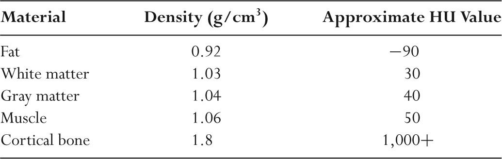
TABLE 5.3 Hounsfield Units (HU) for Representative Materials

C. Hounsfield units

–CT images are maps of the relative linear attenuation values of tissues.

–The relative attenuation coefficient (μ) is normally expressed as CT numbers.

–CT numbers are known as Hounsfield units (HU).

–The HU of material x is HU_x = 1,000 × (μ_x − μ_water)/μ_water where μ_x is the attenuation coefficient of the material x and μ_water is the attenuation coefficient of water.

–By definition, the HU value for water is always 0.

–The HU value for air is –1,000 since μ_air is negligible compared to μ_water.

–Table 5.3 lists typical HU values for a range of tissues.

–Because μ_x and μ_water are dependent on photon energy (keV), HU values depend on the kV and filtration.

–HU values generated by a CT scanner are only approximate.

–HU may be used to characterize tissue.

–For example, a HU of –100 suggests that the tissue being examined is fat and a HU of +50 suggests the tissue being examined is muscle.

D. Field of view

–The field of view (FOV) is the diameter of the body region being imaged.

–A head CT normally has a FOV of ~25 cm.

–A body CT normally has a FOV of ~40 cm.

–The matrix size in CT is normally 512 × 512.

–CT pixel size is determined by dividing the FOV by the matrix size.

–Pixel sizes are 0.5 mm for a 25-cm diameter FOV head scan (25 cm divided by 512).

–Pixel sizes are 0.8 mm for a 40-cm FOV body scan (40 cm divided by 512).

–Voxel is a volume element in the patient.

–Voxel volume is the product of the pixel area and slice thickness.

–In the early days of CT, the acquired slice thickness ranged from 1 to 10 mm.

–For MDCT, the acquired slice thickness is generally ~0.5 to ~0.6 mm.

–Figure 5.4 shows voxel and pixel sizes encountered in CT.

–The field of view may be reduced by reducing the fan beam angle.

–Unlike diagnostic x-rays, regions outside of a reduced FOV will receive a direct dose.

E. Image display

–A 35-cm-long chest CT scan, acquired with a 0.5-mm slice thickness, would result in 700 images.

–CT images are normally viewed with a 3-or 5-mm slice thickness, which combines six to 10 thin slices.

–CT images viewed on monitors have a pixel brightness related to the average attenuation coefficient.

–Each pixel is normally represented by 12 bits, or 4,096 gray levels.

–Window width and level optimize the appearance of CT images by determining the contrast and brightness levels assigned to the CT image data.

–Figure 5.5 shows how the choice of window and level value affects the appearance of a given CT number (HU value).

–CT images with a window width of 100 HU and a window level (center) of 50 HU have HU <0 black, HU >100 white, and HU ~50 mid-gray.

–Window (width and level) settings affect only the displayed image, not the reconstructed image data stored in the computer.

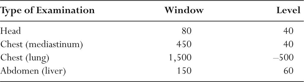
–Table 5.4 shows typical window and level settings used in clinical CT.

–Multiplanar reformatting (MPR) generates coronal, sagittal, or oblique images from the original axial image data.

–Maximum intensity projection (MIP) is useful to visualize tortuous vessels with contrast agent.

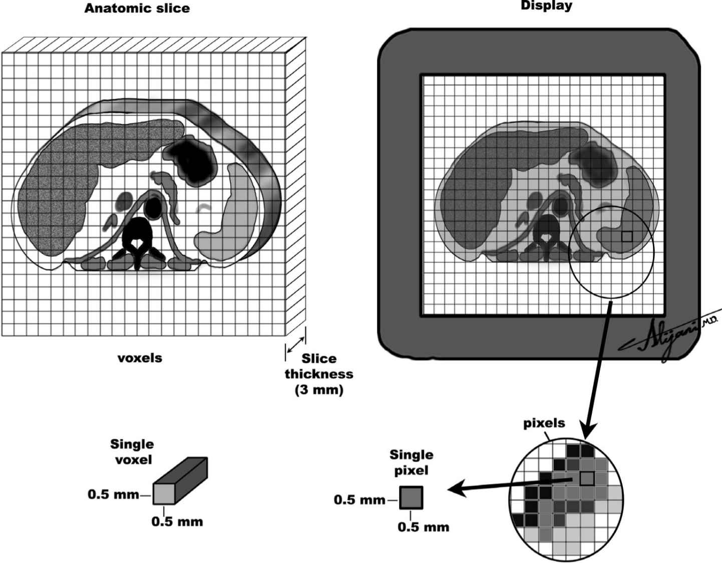
FIGURE 5.4 Schematic representation of an anatomic slice (left) and the corresponding image display (right) showing typical pixels and voxels in CT imaging.

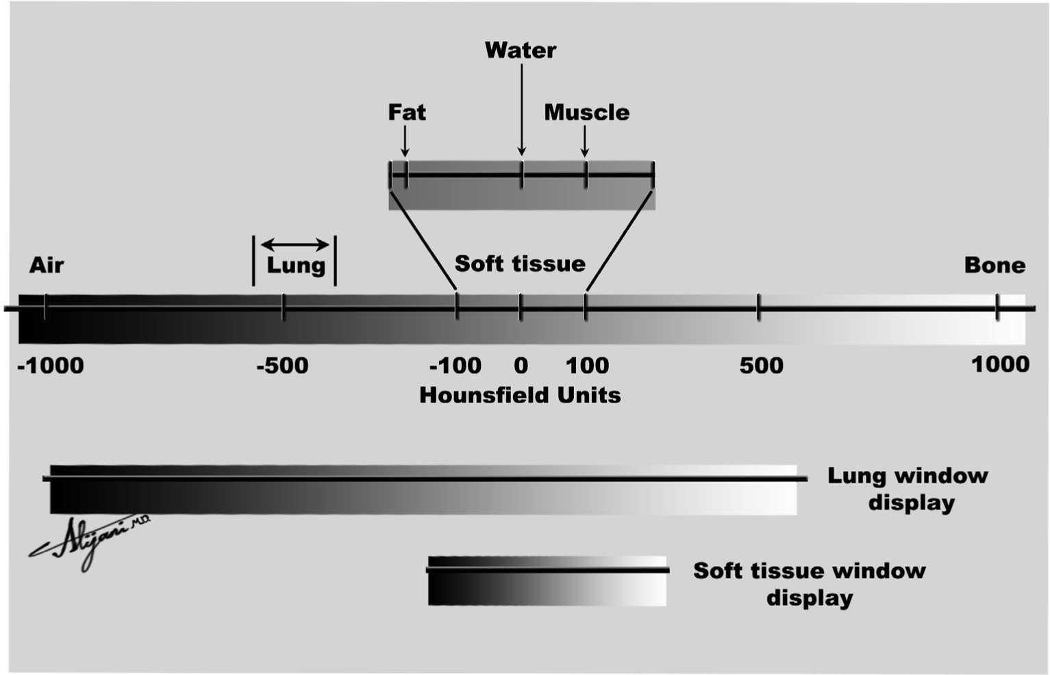
FIGURE 5.5 The CT number scale (Hounsfield unit) ranges from –1,000 to ~+1,000. Its appearance depends on the choice of window level and window width.

TABLE 5.4 Typical Window/Level Settings Used in Clinical CT

–Three-dimensional (3-D) or volume rendering of CT data requires segmentation of the image data to select the tissue or structures of interest.

–Shaded surface display is a method for creating surface renderings that simulate a lighted object.

III. SCANNER OPERATION

A. Acquisition geometry

–In 1972, the EMI scanner was the first CT scanner introduced into clinical practice.

–EMI scanners used a pencil beam and sodium iodide (NaI) detectors that moved across the patient (i.e., translated) to obtain one projection data set.

–The x-ray tube and detector were rotated 1 degree, and another projection was obtained (rotation).

–The EMI scanner thus used a translate/rotate acquisition geometry, which is known as a first-generation system.

–The CT scanner generation defines the acquisition geometry.

–An old generation is not (necessarily) inferior.

–Second-generation scanners also use translate-rotate technology but have multiple detectors and a fan-shaped beam.

–Third-generation scanners use a wide rotating fan beam coupled with a large array of detectors (rotate-rotate system).

–The geometric relationship between the tube and detectors does not change as it rotates 360 degrees around the patient.

–Fourth-generation scanners have a rotating tube and fixed ring of detectors (up to 4,800) in the gantry (rotate-fixed system).

–For single-slice CT scanners, third-and fourth-generation acquisition geometries resulted in similar patient doses and image quality.

–

Only gold members can continue reading. Log In or Register to continue