of mutually orthogonal axes x, y and z, represented by unit vectors ![$${\hat{\mathbf{e}}}_{Ix} = [1,0,0]_{I}$$](/wp-content/uploads/2016/12/A312884_1_En_8_Chapter_IEq2.gif) ,
, ![$${\hat{\mathbf{e}}}_{Iy} = [0,1,0]_{I}$$](/wp-content/uploads/2016/12/A312884_1_En_8_Chapter_IEq3.gif) and
and ![$${\hat{\mathbf{e}}}_{Iz} = [0,0,1]_{I}$$](/wp-content/uploads/2016/12/A312884_1_En_8_Chapter_IEq4.gif) , respectively. In the case of 3D spine images, the image-based coordinate system usually corresponds to the coordinate system of the imaging device (i.e. CT or MR scanner), in which the body is longitudinally aligned. The image-based coordinate system is, in general, aligned with the coordinate system of the body, and therefore its axes represent the following anatomical directions:
, respectively. In the case of 3D spine images, the image-based coordinate system usually corresponds to the coordinate system of the imaging device (i.e. CT or MR scanner), in which the body is longitudinally aligned. The image-based coordinate system is, in general, aligned with the coordinate system of the body, and therefore its axes represent the following anatomical directions:
the sinistro–dexter axis x represents the direction from the left to the right part of the body,
the ventro–dorsal axis y represents the direction from the anterior to the posterior part of the body,
the cranio–caudal axis z represents the direction from the superior to the inferior part of the body (i.e. the longitudinal axis of the body).
As a result, the following three imaging planes can be defined:
a sagittal or lateral plane is any plane that passes from the anterior to the posterior, and from the superior to the inferior part of the body, therefore dividing the body into left and right sections (the sagittal plane that passes through the midline of the body and, assuming bilateral symmetry, divides the body into left and right halves is the mid-sagittal plane),
a coronal or frontal plane is any plane that passes from the left to the right, and from the superior to the inferior part of the body, therefore dividing the body into anterior and posterior sections (the coronal plane that passes through the midline of the body and, assuming bilateral symmetry, divides the body into anterior and posterior halves is the mid-coronal plane),
an axial or transverse plane is any plane that passes from the left to the right, and from the anterior to the posterior part of the body, therefore dividing the body into superior and inferior sections.
The image-based coordinate system is therefore a right-handed Cartesian coordinate system with a standard orthonormal basis (Fig. 1).
Fig. 1
The image-based coordinate system  of a 3D image of a scoliotic spine, shown in a 3D view, b left sagittal view, c posterior coronal view and d superior axial view
of a 3D image of a scoliotic spine, shown in a 3D view, b left sagittal view, c posterior coronal view and d superior axial view2.1.2 Spine-Based Coordinate System
The spine-based coordinate system [84] is the coordinate system of the spine as the observed anatomical structure. In the case of 3D spine images, it is defined by a 3-tuple  of mutually orthogonal axes
  ,
,  and
and  , represented by unit vectors
 ![$${\hat{\mathbf{e}}}_{Su} = [1,0,0]_{S}$$](/wp-content/uploads/2016/12/A312884_1_En_8_Chapter_IEq15.gif) ,
, ![$${\hat{\mathbf{e}}}_{Sv} = [0,1,0]_{S}$$](/wp-content/uploads/2016/12/A312884_1_En_8_Chapter_IEq16.gif) and
and ![$${\hat{\mathbf{e}}}_{Sw} = [0,0,1]_{S}$$](/wp-content/uploads/2016/12/A312884_1_En_8_Chapter_IEq17.gif) , respectively. The spine-based coordinate system is aligned with the spine, and its axes represent the following structural directions:
, respectively. The spine-based coordinate system is aligned with the spine, and its axes represent the following structural directions:
of mutually orthogonal axes , and , represented by unit vectors , and , respectively. The spine-based coordinate system is aligned with the spine, and its axes represent the following structural directions:
the anatomical axis represents the direction
  from the left to the right part of the spine,
the anatomical axis represents the direction
  from the anterior to the posterior part of the spine,
the anatomical axis represents the direction
  from the superior to the inferior part of the spine (i.e. the longitudinal axis of the spine).
As a result, the following three anatomical (structural) planes can be defined:
a sagittal or lateral plane is any plane that passes from the anterior to the posterior, and from the superior to the inferior part of the spine, therefore dividing the spine into left and right sections,
a coronal or frontal plane is any plane that passes from the left to the right, and from the superior to the inferior part of the spine, therefore dividing the spine into anterior and posterior sections,
an axial or transverse plane is any plane that passes from the left to the right, and from the anterior to the posterior part of the spine, therefore dividing the spine into superior and inferior sections.
The spine-based coordinate system is therefore a right-handed Cartesian coordinate system with a standard orthonormal basis (Fig. 2).
Fig. 2
The spine-based coordinate system  of a 3D image of a scoliotic spine, shown in a 3D view, b left sagittal view, c posterior coronal view and d superior axial view (Note The spine corresponds to Fig. 1)
of a 3D image of a scoliotic spine, shown in a 3D view, b left sagittal view, c posterior coronal view and d superior axial view (Note The spine corresponds to Fig. 1)2.2 Definition of the Spine-Based Coordinate System
To define the spine-based coordinate system, two geometrical properties of the spine have to be determined, namely the spine curve (Sect. 2.2.1) and axial vertebral rotation (Sect. 2.2.2), which serve to define the transformation from the image-based to the spine-based coordinate system (Sect. 2.2.3).
2.2.1 Spine Curve
The spine curve  is the curve that follows the curvature of the spine along its entire longitudinal length. If
  is an independent parameter that denotes an arbitrary location on the spine, then
  is the parametrization of the spine curve
  :
:
![$$C{:} \quad {\mathbf{c}}(i) = (c_{x} (i),c_{y} (i),c_{z} (i));\quad i \in [i_{\text{sp}} ,i_{\text{ep}} ],$$](/wp-content/uploads/2016/12/A312884_1_En_8_Chapter_Equ1.gif)
where  and
and  represent the locations on the spine at its start and end point of observation, respectively, and
  ,
,  and
and  represent the sagittal, coronal and axial coordinate, respectively, of the same anatomical reference point at any location
  on the spine in the image-based coordinate system. Although arbitrary anatomical reference points can be chosen (e.g. the centers of the spinal canal), the most established anatomical reference points are the centers of vertebral bodies. For
  observed consecutive vertebrae, let points
  represent the corresponding centers of vertebral bodies. The spine curve
  can be then obtained by continuous interpolation of
  between
  and
and  (Fig. 3).
is the curve that follows the curvature of the spine along its entire longitudinal length. If is an independent parameter that denotes an arbitrary location on the spine, then is the parametrization of the spine curve :(1)
and represent the locations on the spine at its start and end point of observation, respectively, and , and represent the sagittal, coronal and axial coordinate, respectively, of the same anatomical reference point at any location on the spine in the image-based coordinate system. Although arbitrary anatomical reference points can be chosen (e.g. the centers of the spinal canal), the most established anatomical reference points are the centers of vertebral bodies. For observed consecutive vertebrae, let points represent the corresponding centers of vertebral bodies. The spine curve can be then obtained by continuous interpolation of between and (Fig. 3).Fig. 3
The sagittal  , coronal
  and axial
  component of the spine curve
  against the independent parameter
 ![$$i \in [0,1]$$](/wp-content/uploads/2016/12/A312884_1_En_8_Chapter_IEq862.gif) . Labels C7, T1, …, L3 indicate vertebral segments (Note The spine corresponds to Fig. 1)
. Labels C7, T1, …, L3 indicate vertebral segments (Note The spine corresponds to Fig. 1)
, coronal and axial component of the spine curve against the independent parameter . Labels C7, T1, …, L3 indicate vertebral segments (Note The spine corresponds to Fig. 1)For a differentiable curve  , the geometric properties of the curve can be described in terms of differential geometry by the Frenet-Serret frame, which is defined as an orthonormal basis by the unit tangent, normal and binormal vectors to the curve. The unit tangent vector
  represents the direction of the curve that corresponds to increasing values of parameter
  :
:
where  is the tangent vector to the curve
  , obtained as the first derivative of
  with respect to
  , and
, and  denotes the vector norm. The unit normal vector
  represents the deviation of the curve from being a straight line:
where  is the normal vector to the curve
  , obtained as the first derivative of
  with respect to
  , and
, and  denotes the cross vector product. To satisfy the orthonormality of the basis, the unit binormal vector
  is orthogonal to both the unit tangent vector and the unit normal vector:
where  is the binormal vector to the curve
  , obtained as the cross vector product of the first and the second derivative of the curve
  .
.
, the geometric properties of the curve can be described in terms of differential geometry by the Frenet-Serret frame, which is defined as an orthonormal basis by the unit tangent, normal and binormal vectors to the curve. The unit tangent vector represents the direction of the curve that corresponds to increasing values of parameter :(2)
is the tangent vector to the curve , obtained as the first derivative of with respect to , and denotes the vector norm. The unit normal vector represents the deviation of the curve from being a straight line:(3)
is the normal vector to the curve , obtained as the first derivative of with respect to , and denotes the cross vector product. To satisfy the orthonormality of the basis, the unit binormal vector is orthogonal to both the unit tangent vector and the unit normal vector:(4)
is the binormal vector to the curve , obtained as the cross vector product of the first and the second derivative of the curve .The unit tangent vector  and the unit normal vector
  at location
  on curve
  define the osculating plane at that location. The deviation of the curve from being a straight line relative to the osculating plane is measured by the geometrical curvature
  (Fig. 4):
where  is the radius of curvature that represents the radius of the osculating circle in the osculating plane. On the other hand, the deviation of the curve from being a plane curve, represented by the rotation of the unit binormal vector
  about the unit tangent vector
  , is measured by the geometrical torsion
  (Fig. 5):
where  denotes the dot vector product, and
  is the radius of torsion. By using the geometrical curvature and torsion, the resulting Frenet-Serret frame can be written in matrix form as:
![$$\frac{\text{d}}{{{\text{d}}i}}\left[ {\begin{array}{*{20}c} {{\hat{\mathbf{t}}}(i)} \\ {{\hat{\mathbf{n}}}(i)} \\ {{\hat{\mathbf{b}}}(i)} \\ \end{array} } \right] = \left\| {\frac{{{\text{d}}{\mathbf{c}}(i)}}{{{\text{d}}i}}} \right\|\left[ {\begin{array}{*{20}c} 0 & {\kappa (i)} & 0 \\ { - \kappa (i) } & 0 & { \tau (i) } \\ 0 & { - \tau (i) } & 0 \\ \end{array} } \right]\left[ {\begin{array}{*{20}c} {{\hat{\mathbf{t}}}(i)} \\ {{\hat{\mathbf{n}}}(i)} \\ {{\hat{\mathbf{b}}}(i)} \\ \end{array} } \right].$$](/wp-content/uploads/2016/12/A312884_1_En_8_Chapter_Equ7.gif)
and the unit normal vector at location on curve define the osculating plane at that location. The deviation of the curve from being a straight line relative to the osculating plane is measured by the geometrical curvature (Fig. 4):Fig. 4
The geometrical curvature  of the spine curve
  against the independent parameter
 ![$$i \in [0,1]$$](/wp-content/uploads/2016/12/A312884_1_En_8_Chapter_IEq865.gif) . Labels C7, T1, …, L3 indicate vertebral segments (Note The spine corresponds to Fig. 1)
. Labels C7, T1, …, L3 indicate vertebral segments (Note The spine corresponds to Fig. 1)
of the spine curve against the independent parameter . Labels C7, T1, …, L3 indicate vertebral segments (Note The spine corresponds to Fig. 1)(5)
is the radius of curvature that represents the radius of the osculating circle in the osculating plane. On the other hand, the deviation of the curve from being a plane curve, represented by the rotation of the unit binormal vector about the unit tangent vector , is measured by the geometrical torsion (Fig. 5):Fig. 5
The geometrical torsion  of the spine curve
  against the independent parameter
 ![$$i \in [0,1]$$](/wp-content/uploads/2016/12/A312884_1_En_8_Chapter_IEq868.gif) . Labels C7, T1, …, L3 indicate vertebral segments (Note The spine corresponds to Fig. 1)
. Labels C7, T1, …, L3 indicate vertebral segments (Note The spine corresponds to Fig. 1)
of the spine curve against the independent parameter . Labels C7, T1, …, L3 indicate vertebral segments (Note The spine corresponds to Fig. 1)(6)
denotes the dot vector product, and is the radius of torsion. By using the geometrical curvature and torsion, the resulting Frenet-Serret frame can be written in matrix form as:(7)
The form of Eqs. 2–7 corresponds to a regular parametrization of the curve by location i on the curve (Eq. 1). In the case the curve is reparameterized by its arc length s, the natural parametrization  of
of  is yielded:
of is yielded:(8)
Considering the natural parametrization of the curve, the unit tangent vector  , unit normal vector
  and unit binormal vector
  are computed as:
the corresponding geometrical curvature  and torsion
  are computed as:
and the Frenet-Serret frame in the matrix form is:
![$$\frac{\text{d}}{\text{d}{s}}\left[ {\begin{array}{*{20}c} {{\hat{\mathbf{t}}}(s)} \\ {{\hat{\mathbf{n}}}(s)} \\ {{\hat{\mathbf{b}}}(s)} \\ \end{array} } \right] = \left[ {\begin{array}{*{20}c} 0 & {\kappa (s)} & 0 \\ { - \kappa (s) } & 0 & { \tau (s) } \\ 0 & { - \tau (s) } & 0 \\ \end{array} } \right]\left[ {\begin{array}{*{20}c} {{\hat{\mathbf{t}}}(s)} \\ {{\hat{\mathbf{n}}}(s)} \\ {{\hat{\mathbf{b}}}(s)} \\ \end{array} } \right].$$](/wp-content/uploads/2016/12/A312884_1_En_8_Chapter_Equ11.gif)
, unit normal vector and unit binormal vector are computed as:(9)
and torsion are computed as:(10)
(11)
However, the natural parametrization is in the case of spine curves rare, as it is often based on the axial coordinate  at the start and end point of the spine curve (i.e.
  and
and  , where
  is the start point and
  is the end point), or on pre-defined constant values (e.g.
  and
and  ).
).
at the start and end point of the spine curve (i.e. and , where is the start point and is the end point), or on pre-defined constant values (e.g. and ).2.2.2 Axial Vertebral Rotation
Axial vertebral rotation is the rotation  of vertebrae around their longitudinal axes when projected onto the transverse plane of the corresponding coordinate system. If
  is an independent parameter that denotes an arbitrary location on the spine, then
  is the parametrization of the axial vertebral rotation
  :
:
![$${\varPhi } {:} \quad \varphi (i);\quad i \in [i_{\text{sp}} ,i_{\text{ep}} ],$$](/wp-content/uploads/2016/12/A312884_1_En_8_Chapter_Equ12.gif)
where  and
and  represent the locations on the spine at its start and end point of observation, respectively. For
  observed consecutive vertebrae, let angles
  represent the corresponding axial vertebral rotation angles. The axial vertebral rotation
  can be then obtained by continuous interpolation of
  between
  and
and  (Fig. 6).
of vertebrae around their longitudinal axes when projected onto the transverse plane of the corresponding coordinate system. If is an independent parameter that denotes an arbitrary location on the spine, then is the parametrization of the axial vertebral rotation :(12)
and represent the locations on the spine at its start and end point of observation, respectively. For observed consecutive vertebrae, let angles represent the corresponding axial vertebral rotation angles. The axial vertebral rotation can be then obtained by continuous interpolation of between and (Fig. 6).Fig. 6
The axial vertebral rotation  against the independent parameter
 ![$$i \in [0,1]$$](/wp-content/uploads/2016/12/A312884_1_En_8_Chapter_IEq870.gif) . Labels C7, T1, …, L3 indicate vertebral segments (Note The spine corresponds to Fig. 1)
. Labels C7, T1, …, L3 indicate vertebral segments (Note The spine corresponds to Fig. 1)
against the independent parameter . Labels C7, T1, …, L3 indicate vertebral segments (Note The spine corresponds to Fig. 1)Axial vertebral rotation cannot be uniformly measured, as the vertebral anatomy observed in the transverse plane is not completely symmetrical due to normal developmental as well as pathological conditions affecting the spine. As a result, several methods were developed to determine axial vertebral rotation from 3D images of the spine [88] that measured the angle between the reference sagittal plane and a line connecting specific anatomical reference points in the transverse plane. For example, axial vertebral rotation was measured as the angle between the reference sagittal plane and the line connecting the posterior junction of the two laminae of the vertebral arch with the center of vertebral body [1], as the angle between the reference sagittal plane and the line bisecting the angle between the two lines connecting the junction of each lamina and the pedicle with the posterior junction of the two laminae [26], as the angle between the reference sagittal plane and the line connecting the tip of the spinous process with the center of vertebral body [39], or as the angle between the reference sagittal plane and the line connecting the most posterior points of the two pedicles [20].
Let points  represent locations of the selected anatomical reference points in the corresponding transverse planes of measurement, and let
  represent the spine curve that passes through the centers of vertebral bodies. If the transverse planes of measurement are image-based, i.e. orthogonal to axis
  of the image-based coordinate system, then the axial vertebral rotation
  can be determined by considering
  as:
as:
which for every  corresponds to the angle between the line connecting the anatomical reference point with the center of the vertebral body, and the line representing the reference sagittal plane (i.e. the line in the direction of axis
  of the image-based coordinate system). However, because vertebrae can be sagittally or coronally inclined against axis
  , the centers of vertebral bodies and the corresponding reference anatomical points may not represent corresponding anatomical locations along the longitudinal vertebral axes. On the other hand, if the transverse planes of measurement are spine-based, i.e. orthogonal to axis
  of the spine-based coordinate system and therefore orthogonal to
  , then the axial vertebral rotation
  is measured at corresponding anatomical locations and can be determined as:
where  is the unit vector in the direction of the projection of
 ![$${\hat{\mathbf{e}}}_{Iy} = [0,1,0]_{I}$$](/wp-content/uploads/2016/12/A312884_1_En_8_Chapter_IEq110.gif) to the plane orthogonal to the spine curve, defined by the unit tangent vector
to the plane orthogonal to the spine curve, defined by the unit tangent vector  as the normal of that plane.
represent locations of the selected anatomical reference points in the corresponding transverse planes of measurement, and let represent the spine curve that passes through the centers of vertebral bodies. If the transverse planes of measurement are image-based, i.e. orthogonal to axis of the image-based coordinate system, then the axial vertebral rotation can be determined by considering as:(13)
corresponds to the angle between the line connecting the anatomical reference point with the center of the vertebral body, and the line representing the reference sagittal plane (i.e. the line in the direction of axis of the image-based coordinate system). However, because vertebrae can be sagittally or coronally inclined against axis , the centers of vertebral bodies and the corresponding reference anatomical points may not represent corresponding anatomical locations along the longitudinal vertebral axes. On the other hand, if the transverse planes of measurement are spine-based, i.e. orthogonal to axis of the spine-based coordinate system and therefore orthogonal to , then the axial vertebral rotation is measured at corresponding anatomical locations and can be determined as:(14)
is the unit vector in the direction of the projection of to the plane orthogonal to the spine curve, defined by the unit tangent vector as the normal of that plane.2.2.3 Transformation from Image-Based to Spine-Based Coordinate System
The continuous transformation from the image-based coordinate system (Fig. 7) to the spine-based coordinate system (Fig. 8) is possible by having a continuous description of the spine curve  (Eq. 1) and axial vertebral rotation
  (Eq. 12) that are parameterized by the same variable
  representing the location on the spine:
![$$\{ C, {\varPhi } \} {:} \quad \zeta (i) = ({\mathbf{c}}(i),\varphi (i)) = (c_{x} (i),c_{y} (i),c_{z} (i),\varphi (i));\quad i = [i_{\text{sp}} ,i_{\text{ep}} ],$$](/wp-content/uploads/2016/12/A312884_1_En_8_Chapter_Equ15.gif)
where  and
and  represent the locations of the spine curve and axial vertebral rotation at the start and end point of observation on the spine, respectively.
(Eq. 1) and axial vertebral rotation (Eq. 12) that are parameterized by the same variable representing the location on the spine:Fig. 7
The spine curve (red line) and axial vertebral rotation (blue directions) in the image-based coordinate system  of a 3D image of a scoliotic spine, shown in a 3D view, b left sagittal view, c posterior coronal view and d superior axial view. The spine curve is defined between the start point
  and end point
  , while the coordinates are shown also for a selected point
  on the spine curve
of a 3D image of a scoliotic spine, shown in a 3D view, b left sagittal view, c posterior coronal view and d superior axial view. The spine curve is defined between the start point and end point , while the coordinates are shown also for a selected point on the spine curveFig. 8
The spine curve (red line) and axial vertebral rotation (blue directions) in the spine-based coordinate system  of a 3D image of a scoliotic spine, shown in a 3D view, b left sagittal view, c posterior coronal view and d superior axial view. The spine curve is defined between the start point
  and end point
  , while the coordinates are shown also for a selected point
  on the spine curve
of a 3D image of a scoliotic spine, shown in a 3D view, b left sagittal view, c posterior coronal view and d superior axial view. The spine curve is defined between the start point and end point , while the coordinates are shown also for a selected point on the spine curve(15)
and represent the locations of the spine curve and axial vertebral rotation at the start and end point of observation on the spine, respectively.The Frenet-Serret frame (Eq. 7) describes the geometrical properties of the curve and can be therefore applied to the spine curve  . However, the spine-based coordinate system
  has to represent also the course of the axial vertebral rotation
  . The unit tangent vector
  defines the unit vector
 ![$${\hat{\mathbf{e}}}_{Sw} = [0,0,1]_{S}$$](/wp-content/uploads/2016/12/A312884_1_En_8_Chapter_IEq121.gif) representing axis
representing axis  at any point
  on the spine curve. At the same time it defines, as the normal, the plane orthogonal to the spine curve at any point
  , which is the plane that contains unit vectors
 ![$${\hat{\mathbf{e}}}_{Su} = [1,0,0]_{S}$$](/wp-content/uploads/2016/12/A312884_1_En_8_Chapter_IEq125.gif) and
and ![$${\hat{\mathbf{e}}}_{Sv} = [0,1,0]_{S}$$](/wp-content/uploads/2016/12/A312884_1_En_8_Chapter_IEq126.gif) representing axes
representing axes  and
and  , respectively. However,
  and
and  do not correspond to the unit normal vector
  or unit binormal vector
  , although they lie in the same plane, i.e. the plane orthogonal to the spine curve, because
  and
and  rotate about
  as described by the geometrical torsion
  . The directions of
  and
and  are namely defined by the axial vertebral rotation
  . If
. If  (Eq. 13), meaning that the axial vertebral rotation is defined in transverse planes of measurement that are orthogonal to axis
  of the image-based coordinate system, then the modified unit normal vector
  equals:
where matrix  represents the rotation for angle
  about axis
  of the image-based coordinate system:
![$$R_{z} (\varphi_{z} (i)) = \left[ {\begin{array}{*{20}c} {\cos \varphi_{z} (i)} & { - \sin \varphi_{z} (i)} & 0 \\ {\sin \varphi_{z} (i)} & ~~~~{\cos \varphi_{z} (i)} & 0 \\ {\;\;\;\,0} & {\;\;\,0} & 1 \\ \end{array} } \right],$$](/wp-content/uploads/2016/12/A312884_1_En_8_Chapter_Equ17.gif)
with the center of rotation at point  . On the other hand, if
  (Eq. 14), meaning that the axial vertebral rotation is defined in transverse planes of measurement that are orthogonal to the spine curve
  , then the modified unit normal vector
  equals:
where  is the unit vector in the direction of the projection of
 ![$${\hat{\mathbf{e}}}_{Iy} = [0,1,0]_{I}$$](/wp-content/uploads/2016/12/A312884_1_En_8_Chapter_IEq151.gif) to the plane orthogonal to the spine curve (Eq. 14), and matrix
to the plane orthogonal to the spine curve (Eq. 14), and matrix  represents the rotation for angle
  about the axis defined by the unit tangent vector
  :
:
![$$\begin{aligned} R_{{{\hat{\mathbf{t}}}(i)}} (\varphi_{w} (i)) & = \cos (\varphi_{w} (i)) I_{3} \\ & \quad + \sin (\varphi_{w} (i)) [{\hat{\mathbf{t}}}(i)]_{ \times } \\ & \quad + (1 - \cos (\varphi_{w} (i))) [{\hat{\mathbf{t}}}(i) \otimes {\hat{\mathbf{t}}}(i)], \\ \end{aligned}$$](/wp-content/uploads/2016/12/A312884_1_En_8_Chapter_Equ19.gif)
with the center of rotation at point  . In Eq. 19,
  denotes the identity matrix of size
  , and
, and ![$$[{\hat{\mathbf{t}}}(i)]_{ \times }$$](/wp-content/uploads/2016/12/A312884_1_En_8_Chapter_IEq158.gif) and
and ![$$[{\hat{\mathbf{t}}}(i){\kern 1pt} \otimes {\kern 1pt} {\hat{\mathbf{t}}}(i)]$$](/wp-content/uploads/2016/12/A312884_1_En_8_Chapter_IEq159.gif) are, respectively, the cross and tensor product matrix of
are, respectively, the cross and tensor product matrix of  :
:
![$$[{\hat{\mathbf{t}}}(i)]_{ \times } = \left[ {\begin{array}{*{20}c} ~~~0 & { - \hat{t}_{z} (i) } & ~~~{ \hat{t}_{y} (i) } \\ ~~~{ \hat{t}_{z} (i) } & 0 & { - \hat{t}_{x} (i) } \\ { - \hat{t}_{y} (i) } & ~~~{ \hat{t}_{x} (i) } & ~~~0 \\ \end{array} } \right],$$](/wp-content/uploads/2016/12/A312884_1_En_8_Chapter_Equ20.gif)
![$$[{\hat{\mathbf{t}}}(i) \otimes {\hat{\mathbf{t}}}(i)] = \left[ {\begin{array}{*{20}c} { (\hat{t}_{x} (i))^{2} } & { \hat{t}_{x} (i){\kern 1pt} \hat{t}_{y} (i) } & { \hat{t}_{x} (i){\kern 1pt} \hat{t}_{z} (i) } \\ { \hat{t}_{x} (i){\kern 1pt} \hat{t}_{y} (i) } & { (\hat{t}_{y} (i))^{2} } & { \hat{t}_{y} (i){\kern 1pt} \hat{t}_{z} (i) } \\ { \hat{t}_{x} (i){\kern 1pt} \hat{t}_{z} (i) } & { \hat{t}_{y} (i){\kern 1pt} \hat{t}_{z} (i) } & { (\hat{t}_{z} (i))^{2} } \\ \end{array} } \right].$$](/wp-content/uploads/2016/12/A312884_1_En_8_Chapter_Equ21.gif)
. However, the spine-based coordinate system has to represent also the course of the axial vertebral rotation . The unit tangent vector defines the unit vector representing axis at any point on the spine curve. At the same time it defines, as the normal, the plane orthogonal to the spine curve at any point , which is the plane that contains unit vectors and representing axes and , respectively. However, and do not correspond to the unit normal vector or unit binormal vector , although they lie in the same plane, i.e. the plane orthogonal to the spine curve, because and rotate about as described by the geometrical torsion . The directions of and are namely defined by the axial vertebral rotation . If (Eq. 13), meaning that the axial vertebral rotation is defined in transverse planes of measurement that are orthogonal to axis of the image-based coordinate system, then the modified unit normal vector equals:(16)
represents the rotation for angle about axis of the image-based coordinate system:(17)
. On the other hand, if (Eq. 14), meaning that the axial vertebral rotation is defined in transverse planes of measurement that are orthogonal to the spine curve , then the modified unit normal vector equals:(18)
is the unit vector in the direction of the projection of to the plane orthogonal to the spine curve (Eq. 14), and matrix represents the rotation for angle about the axis defined by the unit tangent vector :(19)
. In Eq. 19, denotes the identity matrix of size , and and are, respectively, the cross and tensor product matrix of :(20)
(21)
In both cases, the unit binormal vector also changes its direction to fit the orthonormal basis, and is therefore equal to  . The resulting axes
  ,
,  and
and  of the spine-based coordinate system are therefore represented by:
![$$u {:} \quad ~~~{\hat{\mathbf{e}}}_{Su} = [1,0,0]_{S} \quad \leftrightarrow \quad {\hat{\mathbf{b}}}_{\varphi } (i),$$](/wp-content/uploads/2016/12/A312884_1_En_8_Chapter_Equ22.gif)
![$$v {:} \quad ~~~{\hat{\mathbf{e}}}_{Sv} = [0,1,0]_{S} \quad \leftrightarrow \quad {\hat{\mathbf{n}}}_{\varphi } (i),$$](/wp-content/uploads/2016/12/A312884_1_En_8_Chapter_Equ23.gif)
![$$w {:} \quad {\hat{\mathbf{e}}}_{Sw} = [0,0,1]_{S} \quad \leftrightarrow \quad {\hat{\mathbf{t}}}(i).$$](/wp-content/uploads/2016/12/A312884_1_En_8_Chapter_Equ24.gif)
. The resulting axes , and of the spine-based coordinate system are therefore represented by:(22)
(23)
(24)
In contrast to the image-based coordinate system, which is defined in the Euclidean space, the spine-based coordinate system is defined in a non-Euclidean space, and therefore morphometric measurements based on Euclidean metrics can not be obtained directly from the spine-based coordinate system.
2.3 Automated Determination of the Spine-Based Coordinate System
The spine-based coordinate system can be manually determined by identifying distinctive anatomical points on each vertebra (e.g. the centers of vertebral bodies) and the corresponding rotation of vertebrae, and then interpolating through these points to obtain a continuous description of both the spine curve and axial vertebral rotation along the whole length of the spine. However, navigation through 3D spine images is time-consuming and subjective, moreover it is practically impossible to manually define the plane orthogonal to the spine curve, in which axial vertebral rotation is defined, basing only on the identified anatomical points on each vertebra. As a result, several automated and semi-automated methods based on image processing and analysis techniques were proposed to determine the spine curve and/or axial vertebral rotation in 3D spine images.
2.3.1 Automated Determination of the Spine Curve
In the past, the only possibility for measuring the geometrical properties of the spine curve was based on examining the antero-posterior and/or lateral radiographs. As a result, the spine curve in 3D was observed as its projection in 2D in the form of coronal and sagittal spinal curvatures. Moreover, these curvatures were usually evaluated by one-dimensional measures including angles of curvature (e.g. the Ferguson angle, the Cobb angle, the tangent line angle) and indices of curvature (e.g. the Greenspan index, the Ishihara index). A detailed review of methods for the determination of spinal curvature was performed by Vrtovec et al. [89].
With the development of 3D imaging techniques, methods that captured the 3D nature of the spine started to emerge, followed by application of computerized techniques that automatically or semi-automatically (i.e. with minimal observer interaction) determined the spine curve in 3D images. Due to the continuous course of the spinal curvature, a number of studies attempted to model the spine curve with a mathematical curve in stereoradiographic (i.e. in multiple radiographs acquired at different angles), CT or MR spine images. Different functions were used for modeling, such as harmonic functions (i.e. sines, cosines or Fourier series) [13, 15, 27, 58, 74], spline functions [6, 33, 55, 82] and standard polynomial functions [56, 83, 85, 86], as well as statistical interpolation techniques, such as kriging [59].
By computerized least-squares aligning of a parametric sine function to the stereographically reconstructed landmarks, Stokes et al. [74] measured the Cobb angle between the normals to the obtained curve at inflection points in the coronal and sagittal plane, and in the plane of maximal curvature. Drerup and Hierholzer [13–15] also considered the sine function appropriate, as it most resembled the appearance of curves in idiopathic scoliosis. On the other hand, Patwardhan et al. [55] justified the use of spline functions by stating that splines are used to describe geometries with continuously changing curvature, such as scoliotic spines. In their framework for spine segmentation from CT images, Kaminsky et al. [33] used spline functions because they proved appropriate to describe both the anatomical shape and scoliotic deformations of the spine. Berthonnaud and Dimnet [6] constructed the spine curve separately in coronal and sagittal projections by computing the average of two spline functions that connected the anatomical landmarks on vertebral body walls. On the other hand, Peng et al. [56] used polynomial functions to detect and segment vertebrae from MR images using vertebral disc templates. Polynomial functions were also used to model both normal and pathological spine curves in CT images by Vrtovec et al. [83]. The spine curve was automatically determined by aligning the polynomial function with the centers of vertebral bodies in 3D, obtained by maximizing the distance from the edges of vertebral bodies. The same authors also developed a method for MR images [86], where the center of vertebral body was first automatically detected in each axial cross-section by maximizing the entropy of image intensities inside a circular region, and the detected centers of vertebral bodies in 3D were then joined by a polynomial function using the robust least-trimmed-squares regression. The method was also used by Neubert et al. [49] for extracting the spine curve from MR images of high resolution, obtained by applying the sequence named sampling perfection with application optimized contrasts using different flip angle evolution (SPACE). The work was continued by Štern et al. [78], who proposed a modality-independent method for the determination of the spine curve that was extracted from locations where lines connecting opposite edge points on vertebral body walls in the direction of corresponding image intensity gradients most often intersected. Kadoury et al. [30, 31] determined the spine curve of a scoliotic spine in biplanar radiographs by first embedding cubic B-spline functions onto a non-linear manifold to predict an initial curve according to a given database of scoliotic curves, and then performing analytical regression to obtain a statistical model of the final curve.
To extract the spinal canal centerline from CT images, Yao et al. [96] applied a watershed algorithm followed by a graph search, while Hay et al. [24] applied the fast marching minimal path technique that was based on the distance transform of the spinal canal segmentation, obtained by morphological region growing. On the other hand, Klinder et al. [36] segmented the spinal canal by a progressive adaptation of small tubular segments, represented as triangulated surface meshes, and then determined the spinal canal centerline by calculating the centers of mass for all contours of the obtained tubular mesh. A similar approach was proposed by Forsberg et al. [17, 18], who extracted the spinal canal centerline in CT images by first modeling the vertebral foramen in 2D axial cross-sections with circles, and then fitting a cubic B-spline function to the centers of the obtained circles.
Besides modeling the spine curve in 3D, different geometrical descriptors of spinal curvature were derived from mathematical functions. Poncet et al. [58] proposed the geometrical torsion as a measure for classifying spinal deformities, and Kadoury et al. [29, 32] further showed that it can be potentially used to discriminate among different types of thoracolumbar deformations of the spine. Vrtovec et al. [85] showed that clinically relevant features of the spine can be identified in 3D by observing the geometrical curvature as well as the curvature angle, which was defined as the angular magnitude of the geometrical curvature on an arbitrary spine section, and was as such independent of the size of the spine. Hay et al. [24] observed both the geometrical curvature and geometrical torsion that were scaled to a subject-independent coordinate system, and showed that they can be used to detect and quantify pathological spinal curvatures.
2.3.2 Automated Determination of the Axial Vertebral Rotation
Similarly as for the spinal curvature, measurements of axial vertebral rotation were in the past possible only by examining the location of pedicles and spinous processes in relation to corresponding vertebral bodies in antero-posterior radiographs. As a result, the axial vertebral rotation in 3D was observed as its projection in 2D, and several methods based on indices (e.g. the Cobb method, the Nash-Moe method, the Fait-Janovec method) or actual angles (e.g. the Bunnell method, the Drerup method, the Stokes et al. method) were proposed. With the introduction of 3D imaging techniques, cross-sectional imaging in the axial plane became possible and stimulated the development of methods that were based on manual identification of distinctive anatomical reference points (e.g. the tip of spinous process, the center of the vertebral body, etc.). A detailed review of methods for the determination of axial vertebral rotation was performed by Lam et al. [40] and Vrtovec et al. [88].
The measurement of axial vertebral rotation was also approached by computerized techniques based on image processing and analysis, although manual initialization was still required. Haughton et al. [23] and Rogers et al. [66, 67] proposed a method that required manual determination of the axial CT [66] or MR [23, 67] cross-section, the center of rotation and the circular area that encompassed the observed lumbar vertebra. After initialization, the method automatically measured the axial vertebral rotation relative to the cross-section of a different vertebra by searching for the maximal correlation of image intensities between the circular areas determined in both cross-sections. Oblique CT cross-sections were used by Adam and Askin [2], who determined the axial vertebral rotation from the line that bisected the thresholded image of the vertebral body according to the symmetry ratio, defined by the maximal correlation of image intensities in the bisected regions. Kouwenhoven et al. [37, 38] manually selected axial cross-sections through the centers of vertebral bodies in CT [38] and MR [37] images of normal spines, and applied automated region growing segmentation to obtain reference points, such as the center of the vertebral canal, the center of the sternum at the T5 vertebra and the center of the anterior half of the vertebral body, which were used to define the axial vertebral rotation. Axial vertebral rotation was studied in both CT and MR images of whole spines also by Vrtovec et al. [83, 86]. In CT images [83], circular cross-sections that were orthogonal to the spine curve were first automatically extracted, and axial vertebral rotation was then defined from the line that bisected the cross-section and resulted in the maximal correlation of image intensities in the bisected regions. For MR images [86], the rotation was defined in an optimization procedure that searched for the orientation angle of the line of symmetry in each axial-cross section, and then smoothed with a polynomial function along the whole spine using the least-trimmed-squares regression technique. The same authors also combined both approaches into a method that was modality-independent, i.e. applicable to both CT and MR images [87]. Basing on the pre-defined location of the vertebral body center in 3D, they obtained the relation between the image-based and vertebra-based coordinate systems by matching image intensity gradients that defined the best available symmetry of vertebral anatomical structures. The method was thoroughly evaluated and compared to established manual methods when applied to CT [91] and MR [90] images of normal and scoliotic spines. To segment vertebral bodies in both CT and MR images, Štern et al. [79] proposed to use a parametric model based on superquadrics that, among several shape parameters, included also the axial rotation of the vertebral body, and which was later used to perform quantitative vertebral morphometry in CT images of normal and fractured vertebrae [80]. Axial vertebral rotation was determined from the symmetry of vertebral anatomical structures also in the study of Forsberg et al. [18], who for each vertebra in CT images extracted a cross-section that was orthogonal to the spine curve and passed through the center of the vertebral body, and then minimized the sum of absolute differences in image intensities over the line that bisected the cross-section at the evaluated rotation angle. The same group of authors also developed a method for segmentation of vertebrae by registering a spine model to CT spine images, and then measured axial vertebral rotation from landmarks that were placed at distinctive anatomical locations in the spine model and mapped to each CT image by using the obtained registration transformation fields [17].
2.3.3 Examples of Automated Determination of the Spine Curve and Axial Vertebral Rotation
Among automated methods for the determination of the spine curve  and/or axial vertebral rotation
  , the following approaches are presented in detail:
and/or axial vertebral rotation , the following approaches are presented in detail:
automated determination of the spine curve and axial vertebral rotation in CT images [83] (section Automated Determination of the Spine Curve and Axial Vertebral Rotation in CT Images),
automated determination of the spine curve and axial vertebral rotation in MR images [86] (section Automated Determination of the Spine Curve and Axial Vertebral Rotation in MR Images),
automated modality–independent determination of the spine curve and axial vertebral rotation in 3D images [78, 83, 86] (section Automated Modality-Independent Determination of the Spine Curve and Axial Vertebral Rotation in 3D Images).
In all of the presented approaches [78, 83, 86], the spine-based coordinate system is determined from 3D spine images of normal and scoliotic subjects by parameterizing the spine curve  and axial vertebral rotation
  with polynomial functions:
where  ,
,  and
and  are the parameters of polynomial functions
  ,
,  and
and  of degrees
  ,
,  and
and  , respectively, corresponding to the spine curve
  , and
, and  are the parameters of the polynomial function
  of the degree
  corresponding to the axial vertebral rotation
  . The normalization coefficients
  :
:
where  and
and  represent the locations on the spine at its start and end point of observation, respectively, regularize the impact of each polynomial parameter to the absolute variation of the corresponding term. With such parametrization, the goal is to automatically determine polynomial parameters
  that describe the spine curve
  , and polynomial parameters
  that define the axial vertebral rotation
  in the given 3D spine image.
and axial vertebral rotation with polynomial functions:(25)
(26)
, and are the parameters of polynomial functions , and of degrees , and , respectively, corresponding to the spine curve , and are the parameters of the polynomial function of the degree corresponding to the axial vertebral rotation . The normalization coefficients :(27)
and represent the locations on the spine at its start and end point of observation, respectively, regularize the impact of each polynomial parameter to the absolute variation of the corresponding term. With such parametrization, the goal is to automatically determine polynomial parameters that describe the spine curve , and polynomial parameters that define the axial vertebral rotation in the given 3D spine image.Moreover, it is assumed that the 3D image is cropped to a volume of interest according to the start and end point of observation along axis  of the image-based coordinate system, so that the resulting cropped 3D image contains only axial cross-sections that display the observed anatomy of the spine. Although the presented examples may be therefore labeled as semi-automated, manual determination of the volume of interest does not represent a very demanding or time-consuming task. An advantage of such an assumption is that the parametrization of the spine curve and axial vertebral rotation can be based on axial pixel coordinates
  at the start and end point of observation, resulting in
  and
and  , respectively, with the corresponding number of samples equal to
  , where
  is the number of axial cross-sections in the 3D image. Such parametrization is, considering the usual in-plane resolution and slice thickness of CT and MR spine images, in general sufficient for a smooth and continuous description of the spine curve
  and axial vertebral rotation
  .
.
of the image-based coordinate system, so that the resulting cropped 3D image contains only axial cross-sections that display the observed anatomy of the spine. Although the presented examples may be therefore labeled as semi-automated, manual determination of the volume of interest does not represent a very demanding or time-consuming task. An advantage of such an assumption is that the parametrization of the spine curve and axial vertebral rotation can be based on axial pixel coordinates at the start and end point of observation, resulting in and , respectively, with the corresponding number of samples equal to , where is the number of axial cross-sections in the 3D image. Such parametrization is, considering the usual in-plane resolution and slice thickness of CT and MR spine images, in general sufficient for a smooth and continuous description of the spine curve and axial vertebral rotation .Automated Determination of the Spine Curve and Axial Vertebral Rotation in CT Images
Vrtovec et al. [83] proposed a method for automated determination of the spine curve and axial vertebral rotation in CT images. If the spine curve  is represented by a curve that passes through the centers of vertebral bodies, then its determination can be based on the anatomical property that vertebral bodies are locally the largest bone structures of the spine, and on the geometrical property that the center of each vertebral body is represented by the point that is most distant from corresponding edges of the vertebral body. To obtain a quantitative representation of these properties, a distance transform function based on Euclidean metrics is applied twice to image
  , resulting in distance map
  :
:
where  and
and  are the Euclidean distances between the observed point
  and point
  , which represents the closest point to
  with
with  and
and  , respectively. The image intensity threshold
  , which separates the bone structures from the background, can be in the case of CT images determined from the corresponding Hounsfield values. Each value at point
  in the resulting distance map
  , which is of the same size as image
  , represents the Euclidean distance from
  to the edges of the bone structures, and this distance is positive when
  is located inside and negative when
  is located outside the bone structures (Fig. 9). As vertebral bodies are locally the largest bone structures of the spine, distance map values are expected to be the highest in geometrical centers of vertebral bodies and smoothly decrease by moving away from the centers. The optimal polynomial parameters
  that define the spine curve
  (Eq. 25) are finally obtained in an optimization procedure that searches for the combination of parameters that corresponds to the maximal sum of distance map values along the spine curve:
is represented by a curve that passes through the centers of vertebral bodies, then its determination can be based on the anatomical property that vertebral bodies are locally the largest bone structures of the spine, and on the geometrical property that the center of each vertebral body is represented by the point that is most distant from corresponding edges of the vertebral body. To obtain a quantitative representation of these properties, a distance transform function based on Euclidean metrics is applied twice to image , resulting in distance map :(28)
and are the Euclidean distances between the observed point and point , which represents the closest point to with and , respectively. The image intensity threshold , which separates the bone structures from the background, can be in the case of CT images determined from the corresponding Hounsfield values. Each value at point in the resulting distance map , which is of the same size as image , represents the Euclidean distance from to the edges of the bone structures, and this distance is positive when is located inside and negative when is located outside the bone structures (Fig. 9). As vertebral bodies are locally the largest bone structures of the spine, distance map values are expected to be the highest in geometrical centers of vertebral bodies and smoothly decrease by moving away from the centers. The optimal polynomial parameters that define the spine curve (Eq. 25) are finally obtained in an optimization procedure that searches for the combination of parameters that corresponds to the maximal sum of distance map values along the spine curve:Fig. 9
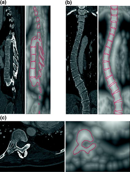
Original image  (left) and the corresponding distance transform
  with superimposed spine boundaries (right), displayed for a selected a sagittal, b coronal and c axial cross-section of a 3D CT image of a scoliotic spine. In the distance transform
  , brighter elements represent positive distances, while darker elements represent negative distances
(left) and the corresponding distance transform with superimposed spine boundaries (right), displayed for a selected a sagittal, b coronal and c axial cross-section of a 3D CT image of a scoliotic spine. In the distance transform , brighter elements represent positive distances, while darker elements represent negative distances(29)
In order to increase the optimization robustness, two additional mechanisms can be applied. First, the amount of information taken into account during optimization can be increased by considering distance map values within a radius from the spine curve, which can be defined from the quantitative morphometrical vertebral analysis [52–54]. Second, optimization can be designed hierarchically and performed on multiple levels. On the first level, the polynomial functions are initialized with degrees of  , i.e. as straight lines. When the optimization reaches the termination criterion, polynomial degrees are increased by
  and the optimization is restarted on the next level, using the polynomial parameters from the previous level for initialization (optionally, the degree of the polynomial function
  can be fixed to
  , therefore always representing a straight line that describes the longitudinal axis of the spine). The maximal polynomial degree can be determined from the flexion points in normal and scoliotic spinal curvatures, as the number of flexion points of a polynomial function is equal to its degree decreased by one (e.g. a straight line is of the first degree and has zero flexion points). For example, when observing the thoracolumbar section of the spine, three distinctive flexion points exist in a normal spinal curvature, i.e. the maximal thoracic kyphosis, the thoracolumbar junction, and the maximal lumbar lordosis, and therefore polynomial functions of the fourth degree represent an adequate choice. Accordingly, a scoliotic spinal curvature can be adequately described by polynomial functions of the fifth degree.
, i.e. as straight lines. When the optimization reaches the termination criterion, polynomial degrees are increased by and the optimization is restarted on the next level, using the polynomial parameters from the previous level for initialization (optionally, the degree of the polynomial function can be fixed to , therefore always representing a straight line that describes the longitudinal axis of the spine). The maximal polynomial degree can be determined from the flexion points in normal and scoliotic spinal curvatures, as the number of flexion points of a polynomial function is equal to its degree decreased by one (e.g. a straight line is of the first degree and has zero flexion points). For example, when observing the thoracolumbar section of the spine, three distinctive flexion points exist in a normal spinal curvature, i.e. the maximal thoracic kyphosis, the thoracolumbar junction, and the maximal lumbar lordosis, and therefore polynomial functions of the fourth degree represent an adequate choice. Accordingly, a scoliotic spinal curvature can be adequately described by polynomial functions of the fifth degree.As the axial vertebral rotation is defined as the rotation of vertebrae about the spine curve, it can be determined automatically in planes that are orthogonal to the spine curve  , defined by polynomial parameters
  (Eq. 29). In each such
  th plane, a circular domain of radius
  and centered at point
  is defined (Fig. 10a). The circular domain is then bisected by a line that passes through the center of the domain and is inclined for angle
  against the projection
  of the unit vector
 ![$${\hat{\mathbf{e}}}_{Iy} = [0,1,0]_{I}$$](/wp-content/uploads/2016/12/A312884_1_En_8_Chapter_IEq228.gif) to the plane (Eq. 14). In the obtained halves
to the plane (Eq. 14). In the obtained halves  and
and  of the
  th circular domain,
  and
and  represent image intensities at mirror pixels according to the line of bisection:
![$$\begin{aligned} s_{A} (i,j,\varphi ) & = I(R_{z} (\varphi ) [ - u,v,c_{z} (i)]) \\ & = I(R_{{{\hat{\mathbf{t}}}(i)}} (\varphi ) [ - x,y,0] + [c_{x} (i),c_{y} (i),c_{z} (i)]), \\ \end{aligned}$$](/wp-content/uploads/2016/12/A312884_1_En_8_Chapter_Equ30.gif)
![$$\begin{aligned} s_{B} (i,j,\varphi ) & = I(R_{z} (\varphi ) [ + u,v,c_{z} (i)]) \\ & = I(R_{{{\hat{\mathbf{t}}}(i)}} (\varphi ) [ + x,y,0] + [c_{x} (i),c_{y} (i),c_{z} (i)]), \\ \end{aligned}$$](/wp-content/uploads/2016/12/A312884_1_En_8_Chapter_Equ31.gif)
where  is the index of the mirror point pair (a total of
  mirror point pairs exist), consecutively assigned on the basis of each
  with
with  , or each
  with
with  (Fig. 10b). Matrices
  (Eq. 17) and
  (Eq. 19) represent, respectively, the rotation1 about axis
  of the spine-based coordinate system and the rotation about the unit tangent vector
  to the spine curve
  at point
  in the image-based coordinate system.
, defined by polynomial parameters (Eq. 29). In each such th plane, a circular domain of radius and centered at point is defined (Fig. 10a). The circular domain is then bisected by a line that passes through the center of the domain and is inclined for angle against the projection of the unit vector to the plane (Eq. 14). In the obtained halves and of the th circular domain, and represent image intensities at mirror pixels according to the line of bisection:Fig. 10
a A circular domain of radius d and centered at the point on the spine curve  , defined in the plane orthogonal to the spine curve
  . b For a bisecting line that is inclined for an angle
  against the direction of
  , image intensities
  and
and  at mirror point pairs are used to evaluate the similarity between the two halves of the circular domain
, defined in the plane orthogonal to the spine curve . b For a bisecting line that is inclined for an angle against the direction of , image intensities and at mirror point pairs are used to evaluate the similarity between the two halves of the circular domain(30)
(31)
is the index of the mirror point pair (a total of mirror point pairs exist), consecutively assigned on the basis of each with , or each with (Fig. 10b). Matrices (Eq. 17) and (Eq. 19) represent, respectively, the rotation1 about axis of the spine-based coordinate system and the rotation about the unit tangent vector to the spine curve at point in the image-based coordinate system.Radius  is defined so that the anatomy of the whole vertebra (and not only of the vertebral body) is captured within the circular domain, and can be defined from the quantitative morphometrical vertebral analysis [52–54]. From the obtained mirror image intensity pairs, the in-plane similarity between the two mirror halves of the
  th circular domain at inclination
  can be quantitatively evaluated by the correlation coefficient
  :
:
where  and
and  are the mean image intensities in parts
  and
and  , respectively, of the circular domain. It is important to note that features other than image intensities can be extracted at mirror points (e.g. image intensity gradients), and similarity measures other than the correlation coefficient can be computed (e.g. mutual information) for the corresponding circular domain halves. Nevertheless, the domain must be circular so that irrespectively of inclination
  , the same points are taken into account for the computation of the in-plane similarity. The optimal polynomial parameters
  that define the axial vertebral rotation
  (Eq. 26) are finally obtained in an optimization procedure that searches for the combination of parameters that corresponds to the maximal sum of correlation coefficients along the spine curve:
is defined so that the anatomy of the whole vertebra (and not only of the vertebral body) is captured within the circular domain, and can be defined from the quantitative morphometrical vertebral analysis [52–54]. From the obtained mirror image intensity pairs, the in-plane similarity between the two mirror halves of the th circular domain at inclination can be quantitatively evaluated by the correlation coefficient :(32)
and are the mean image intensities in parts and , respectively, of the circular domain. It is important to note that features other than image intensities can be extracted at mirror points (e.g. image intensity gradients), and similarity measures other than the correlation coefficient can be computed (e.g. mutual information) for the corresponding circular domain halves. Nevertheless, the domain must be circular so that irrespectively of inclination , the same points are taken into account for the computation of the in-plane similarity. The optimal polynomial parameters that define the axial vertebral rotation (Eq. 26) are finally obtained in an optimization procedure that searches for the combination of parameters that corresponds to the maximal sum of correlation coefficients along the spine curve:(33)
Similarly as in the case of the spine curve, optimization can be designed hierarchically and performed on multiple levels. However, in the case of the axial vertebral rotation, on the first level the optimization starts with a zero degree polynomial, i.e.  , and with polynomial parameter
  , meaning that the initial axial vertebral rotation is constant and equal to zero along the whole length of the spine. When the optimization reaches the termination criterion, the polynomial degree is increased by
  and the optimization is restarted on the next level, using the polynomial parameters from the previous level for initialization. The maximal polynomial degree of
  is adequate for modeling the axial vertebral rotation in both normal and scoliotic spines.
, and with polynomial parameter , meaning that the initial axial vertebral rotation is constant and equal to zero along the whole length of the spine. When the optimization reaches the termination criterion, the polynomial degree is increased by and the optimization is restarted on the next level, using the polynomial parameters from the previous level for initialization. The maximal polynomial degree of is adequate for modeling the axial vertebral rotation in both normal and scoliotic spines.The method was evaluated [83, 85] on  normal and one scoliotic CT image of the thoracolumbar spine, and the reported mean difference between the obtained spine curve in 3D and manually defined ground truth points was
  mm. The performance of the determination of the axial vertebral rotation was, using the sum of absolute differences instead of the correlation coefficient (Eq. 32), evaluated [18] on
  vertebrae extracted from CT images, and the reported mean difference against reference values was around
  with the corresponding 95% confidence interval of around
  .
.
normal and one scoliotic CT image of the thoracolumbar spine, and the reported mean difference between the obtained spine curve in 3D and manually defined ground truth points was mm. The performance of the determination of the axial vertebral rotation was, using the sum of absolute differences instead of the correlation coefficient (Eq. 32), evaluated [18] on vertebrae extracted from CT images, and the reported mean difference against reference values was around with the corresponding 95% confidence interval of around .Automated Determination of the Spine Curve and Axial Vertebral Rotation in MR Images
Vrtovec et al. [86] proposed a method for automated determination of the spine curve and axial vertebral rotation in MR images. The method is based on anatomical properties that vertebral bodies and intervertebral discs are nearly circular in shape and that vertebrae are nearly symmetrical over the lines that pass through the centers of vertebral bodies. In each axial cross-section  of the MR image (Fig. 11a), an arbitrary in-plane line
  that divides the observed cross-section into two image parts, i.e. part
  and part
  , can be defined as:
where  is the slope and
  is the intersection of the line with axis
  of the image-based coordinate system (Fig. 11b). The line that splits the observed cross-section into two symmetrical parts can be obtained by maximizing the similarity between image parts
  and
and  :
:
where  represent all points
  that lie in image parts
  and
and  , respectively, and
  is the similarity measure that can be computed as the standard mutual information between image parts
  and
and  :
:
where  and
and  are the probability distributions of image intensities in image parts
  and
and  , respectively,
  is the joint probability distribution of image intensities, and
  is the number of bins used for probability estimation. The resulting parameters
  and
and  (Eq. 34) define the in-plane line of symmetry, which passes through the center of the vertebral body in the observed
  th axial cross-section.
of the MR image (Fig. 11a), an arbitrary in-plane line that divides the observed cross-section into two image parts, i.e. part and part , can be defined as:Fig. 11
a The search for the line of in-plane symmetry is performed in each ith axial orthogonal multi-planar cross-section of the MR spine image. b The in-plane line  is defined by parameters
  and
and  . c The operator
  is centered in
  and consists of M concentric rings;
  , each with radial width of
  . d The resulting center of the vertebral body
  and in-plane rotation
is defined by parameters and . c The operator is centered in and consists of M concentric rings; , each with radial width of . d The resulting center of the vertebral body and in-plane rotation (34)
is the slope and is the intersection of the line with axis of the image-based coordinate system (Fig. 11b). The line that splits the observed cross-section into two symmetrical parts can be obtained by maximizing the similarity between image parts and :(35)
represent all points that lie in image parts and , respectively, and is the similarity measure that can be computed as the standard mutual information between image parts and :(36)
and are the probability distributions of image intensities in image parts and , respectively, is the joint probability distribution of image intensities, and is the number of bins used for probability estimation. The resulting parameters and (Eq. 34) define the in-plane line of symmetry, which passes through the center of the vertebral body in the observed th axial cross-section.To determine the exact location of the center of the vertebral body, the shape properties of the vertebral anatomy are combined with the appearance of the vertebral body in MR images. When observed in axial cross-sections, the shape of the vertebral body is relatively circular. For a circular structure displayed in a MR image, a certain amount of variation in image intensities is always present along any radial direction, however, in the tangential direction, the variation in image intensities is relatively small. To obtain a quantitative estimation of these properties, the entropy-based operator  is introduced that is centered at an arbitrary point
  and consists of
  concentric rings of radii
  with
with  and radial width of each ring equal to
  (Fig. 11c):
is introduced that is centered at an arbitrary point and consists of concentric rings of radii with and radial width of each ring equal to (Fig. 11c):