(1)
Department of Mathematics and Statistics, Villanova University, Villanova, PA, USA
Electronic supplementary material
The online version of this chapter (doi:10.1007/978-3-319-22665-1_8) contains supplementary material, which is available to authorized users.
8.1 Introduction
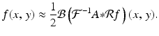
We have seen that, when complete continuous X-ray data are available, then an attenuation-coefficient function f(x, y) can be reconstructed exactly using the filtered back-projection formula, Theorem 6.2. To repeat,
![$$\displaystyle{ f(x,\,y) = \frac{1} {2}\mathcal{B}\left \{\mathcal{F}^{-1}\left [\,\vert S\vert \,\mathcal{F}\left (\mathcal{R}f\,\right )(S,\,\theta )\right ]\right \}(x,\,y). }$$](/wp-content/uploads/2016/10/A183987_2_En_8_Chapter_Equ1.gif)
(8.1)
In Chapter 7, section 7.8, we discussed the practice of replacing the absolute-value function | ⋅ | in (8.1) with a low-pass filter A , obtained by multiplying the absolute value by a window function that vanishes outside some finite interval. Then, in place of (8.1), we use the approximation
(8.2)
The starting point in the implementation of (8.2) in the practical reconstruction of images from X-ray data is that only a finite number of values of  are available in a real study. This raises both questions of accuracy — How many values are needed in order to generate a clinically useful image? — and problems of computation — What do the various components of the formula (8.2) mean in a discrete setting? Also, as we shall see, one step in the algorithm requires essentially that we fill in some missing values. This is done using a process called interpolation that we will discuss later. Each different method of interpolation has its advantages and disadvantages. And, of course, the choice of the low-pass filter affects image quality. (See [45] and [48], from the early days of CT, for concise discussions of these issues.)
are available in a real study. This raises both questions of accuracy — How many values are needed in order to generate a clinically useful image? — and problems of computation — What do the various components of the formula (8.2) mean in a discrete setting? Also, as we shall see, one step in the algorithm requires essentially that we fill in some missing values. This is done using a process called interpolation that we will discuss later. Each different method of interpolation has its advantages and disadvantages. And, of course, the choice of the low-pass filter affects image quality. (See [45] and [48], from the early days of CT, for concise discussions of these issues.)8.2 Sampling
The term sampling refers to the situation where the values of a function that presumably is defined on the whole real line are known or are computed only at a discrete set of points. For instance, we might know the values of the function at all points of the form k ⋅ τ , where τ is called the sample spacing. The basic problem is to determine how many sampled values are enough, or what value τ should have, to form an accurate description of the function as a whole.
For example, consider a string of sampled values {f(k) = 1} , sampled at every integer (so τ = 1 ). These could be the values of the constant function f(x) ≡ 1 , or of the periodic function cos(2π x) . If it is the latter, then we obviously would need more samples to be certain.
Heuristically, we might think of a signal as consisting of a compilation of sine or cosine waves of various frequencies and amplitudes. The narrowest bump in this compilation constitutes the smallest feature that is present in the signal and corresponds to the wave that has the shortest wavelength. The reciprocal of the shortest wavelength present in the signal is the maximum frequency that is present in the Fourier transform of the signal. So this signal is a band-limited function — its Fourier transform is zero outside a finite interval.
Now, suppose that f is a band-limited function for which  whenever | ω | > L. By definition (see (4.7)), the Fourier series coefficients of
  are given by
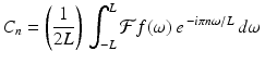
where n is any integer. (Here, we are acting as if  has been extended beyond the interval [−L, L] to be periodic on the real line, with period 2L.) For each integer n, then,
 That is,
 Assuming that
  is continuous, it follows from standard results of Fourier series that
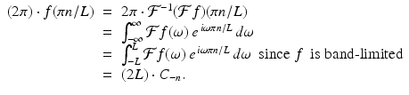
Finally, all of this means that, for every x, we have
![$$\displaystyle\begin{array}{rcl} f(x)& =& \mathcal{F}^{-1}(\mathcal{F}f)(x) {}\\ & =& \left (\frac{1} {2\pi }\right )\,\int _{-L}^{L}\mathcal{F}f(\omega )\,e^{\,i\omega x}\,dx {}\\ & =& \left (\frac{1} {2\pi }\right )\,\left ( \frac{\pi } {L}\right )\,\int _{-L}^{L}\left [\sum _{ n=-\infty }^{\infty }f(\pi n/L)\,e^{\,-in\pi \omega /L}\right ]\,e^{\,i\omega x}\,dx\ \ \mathrm{from\ (8.4)} {}\\ & =& \left ( \frac{1} {2L}\right )\,\sum _{n=-\infty }^{\infty }\left [f(\pi n/L) \cdot \int _{ -L}^{L}e^{\,i\omega (Lx-n\pi )/L}\,d\omega \right ] {}\\ & =& \left ( \frac{1} {2L}\right )\,\sum _{n=-\infty }^{\infty }f(\pi n/L) \cdot (2L) \cdot \left (\frac{\sin (Lx - n\pi )} {Lx - n\pi } \right )\ \mathrm{(Ch.\ 4,\,Exer.\ 4)} {}\\ & =& \sum _{n=-\infty }^{\infty }f(\pi n/L) \cdot \left (\frac{\sin (Lx - n\pi )} {Lx - n\pi } \right ). {}\\ \end{array}$$](/wp-content/uploads/2016/10/A183987_2_En_8_Chapter_Equ6.gif)
whenever | ω | > L. By definition (see (4.7)), the Fourier series coefficients of are given by(8.3)
has been extended beyond the interval [−L, L] to be periodic on the real line, with period 2L.) For each integer n, then, is continuous, it follows from standard results of Fourier series that(8.4)
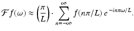
Thus we see that, for a band-limited function f whose Fourier transform vanishes outside the interval [−L, L], the function f can be reconstructed exactly from the values  . In other words, the appropriate sample spacing for the function f is
  . Since L represents the maximum value of | ω | present in the Fourier transform
  , the value 2π∕L represents the smallest wavelength present in the signal f. Therefore, the optimal sample spacing is equal to half of the size of the smallest detail present in the signal. This result is known as Nyquist’s theorem and the value
  is called the Nyquist distance.
. In other words, the appropriate sample spacing for the function f is . Since L represents the maximum value of | ω | present in the Fourier transform , the value 2π∕L represents the smallest wavelength present in the signal f. Therefore, the optimal sample spacing is equal to half of the size of the smallest detail present in the signal. This result is known as Nyquist’s theorem and the value is called the Nyquist distance. To sum up, we have established the following.
Theorem 8.1.
Nyquist’s theorem. If f is a square-integrable band-limited function such that the Fourier transform  whenever |ω| > L, then, for every real number x,
whenever |ω| > L, then, for every real number x,(8.5)
Nyquist’s theorem is also sometimes referred to as Shannon–Whittaker interpolation since it asserts that any value of the function f can be interpolated from the values { f(n π∕L) }.
A heuristic approach to Nyquist’s theorem. As above, assume that the function f is band-limited, with  whenever | ω | > L. We want to extend
  to be periodic on the whole line, so we can take the period to be 2L , the length of the interval − L ≤ ω ≤ L. Now, each of the functions
  , where n is an integer, has period 2L. From the definition of the Fourier transform,
Approximate this integral using a Riemann sum with  . That is, the Riemann sum will use a partition of the line that includes all points of the form n π∕L, where n is an integer. This results in the approximation
 This approximates
  in a way that is periodic on the whole line with period 2L. Notice that this is the same as (8.4) except for having “ ≈ ” instead of “ = .” In the proof above, we appealed to results in the theory of Fourier series that assert that this approximation is actually an equality. Without that knowledge, we instead substitute the approximation for
  into the rest of the proof of Nyquist’s theorem and end up with the approximation

Nyquist’s theorem, which builds on the results concerning Fourier series, asserts that this is in fact an equality.
whenever | ω | > L. We want to extend to be periodic on the whole line, so we can take the period to be 2L , the length of the interval − L ≤ ω ≤ L. Now, each of the functions , where n is an integer, has period 2L. From the definition of the Fourier transform,(8.6)
. That is, the Riemann sum will use a partition of the line that includes all points of the form n π∕L, where n is an integer. This results in the approximation in a way that is periodic on the whole line with period 2L. Notice that this is the same as (8.4) except for having “ ≈ ” instead of “ = .” In the proof above, we appealed to results in the theory of Fourier series that assert that this approximation is actually an equality. Without that knowledge, we instead substitute the approximation for into the rest of the proof of Nyquist’s theorem and end up with the approximation(8.7)
Oversampling. The interpolation formula (8.5) is an infinite series. In practice, we would only use a partial sum. However, the series (8.5) may converge fairly slowly because the expression  is on the order of (1∕n) for large values of n and the harmonic series ∑1∕n diverges. That means that a partial sum might require a large number of terms in order to achieve a good approximation to f(x).
is on the order of (1∕n) for large values of n and the harmonic series ∑1∕n diverges. That means that a partial sum might require a large number of terms in order to achieve a good approximation to f(x).To address this difficulty, notice that, if  whenever | ω | > L, and if R > L, then
  whenever | ω | > R as well. Thus, we can use Shannon–Whittaker interpolation on the interval [−R, R] instead of [−L, L]. This requires that we sample the function f at the Nyquist distance π∕R , instead of π∕L. Since
  , this results in what is called oversampling of the function f. So there is a computational price to pay for oversampling, but the improvement in the results, when using a partial sum to approximate f(x), may be worth that price.
whenever | ω | > L, and if R > L, then whenever | ω | > R as well. Thus, we can use Shannon–Whittaker interpolation on the interval [−R, R] instead of [−L, L]. This requires that we sample the function f at the Nyquist distance π∕R , instead of π∕L. Since , this results in what is called oversampling of the function f. So there is a computational price to pay for oversampling, but the improvement in the results, when using a partial sum to approximate f(x), may be worth that price. 8.3 Discrete low-pass filters
The image reconstruction formula (8.2) involves the inverse Fourier transform  for the low-pass filter A . In practice, this, too, will be sampled, just like the Radon transform. Nyquist’s theorem, Theorem 8.1, tells us how many sampled values are needed to get an accurate representation of
  . Here, we investigate how this works for two particular low-pass filters.
for the low-pass filter A . In practice, this, too, will be sampled, just like the Radon transform. Nyquist’s theorem, Theorem 8.1, tells us how many sampled values are needed to get an accurate representation of . Here, we investigate how this works for two particular low-pass filters.Example 8.2.
![$$\displaystyle\begin{array}{rcl} A(\omega )& =& \vert \omega \vert \cdot \left (\frac{\sin (\pi \omega /(2L))} {\pi \omega /(2L)} \right ) \cdot \sqcap _{L}(\omega ) \\ & =& \left \{\begin{array}{cc} \frac{2L} {\pi } \cdot \left \vert \sin (\pi \omega /(2L))\right \vert &\mbox{ if $\vert \omega \vert \leq L$,} \\ 0 &\mbox{ if $\vert \omega \vert> L$,} \end{array} \right.{}\end{array}$$
” src=”/wp-content/uploads/2016/10/A183987_2_En_8_Chapter_Equ10.gif”></DIV></DIV><br />
<DIV class=EquationNumber>(8.8)</DIV></DIV>for some choice of <SPAN class=EmphasisTypeItalic>L</SPAN> > 0 .</DIV><br />
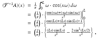
<DIV class=Para>Since <SPAN class=EmphasisTypeItalic>A</SPAN> vanishes outside the interval [−<SPAN class=EmphasisTypeItalic>L</SPAN>, <SPAN class=EmphasisTypeItalic>L</SPAN>] , the inverse Fourier transform of <SPAN class=EmphasisTypeItalic>A</SPAN> is a band-limited function. From the fact that <SPAN class=EmphasisTypeItalic>A</SPAN> is also an even function, we compute, for each real number <SPAN class=EmphasisTypeItalic>x</SPAN> ,<br />
<DIV id=Equ11 class=Equation><br />
<DIV class=EquationContent><br />
<DIV class=MediaObject><IMG alt=](/wp-content/uploads/2016/10/A183987_2_En_8_Chapter_Equ11.gif)
According to Nyquist’s theorem, the function  can be reconstructed exactly from its values taken in increments of the Nyquist distance π∕L . Setting
  in (8.9) yields
![$$\displaystyle\begin{array}{rcl} (\mathcal{F}^{-1}A)(\pi n/L)& =& \left (\frac{L} {\pi ^{2}} \right ) \cdot \left \{\left [ \frac{\cos (\pi n -\pi /2)} {\pi n/L -\pi /(2L)} - \frac{\cos (\pi n +\pi /2)} {\pi n/L +\pi /(2L)}\right ]\right. \\ & & \phantom{Lx +\pi /2bb} -\left.\left [ \frac{1} {\pi n/L -\pi /(2L)} - \frac{1} {\pi n/L +\pi /(2L)}\right ]\right \} \\ & =& \left (\frac{L} {\pi ^{2}} \right ) \cdot \left \{ \frac{1} {\pi n/L +\pi /(2L)} - \frac{1} {\pi n/L -\pi /(2L)}\right \} \\ & =& \frac{4L^{2}} {\pi ^{3}\,(1 - 4n^{2})}. {}\end{array}$$](/wp-content/uploads/2016/10/A183987_2_En_8_Chapter_Equ12.gif)
can be reconstructed exactly from its values taken in increments of the Nyquist distance π∕L . Setting in (8.9) yields(8.10)
Example 8.3.
The Ram–Lak filter, defined in (7.27), has the formula
where the trigonometric identity  was used in the last step.
(8.12)
was used in the last step.As before, set  to evaluate
  at multiples of the Nyquist distance π∕L . Thus,
![$$\displaystyle\begin{array}{rcl} (\mathcal{F}^{-1}A)(\pi n/L)& =& \left (\frac{1} {\pi } \right ) \cdot \left \{\frac{(\pi n) \cdot \sin (\pi n)} {(\pi n/L)^{2}} -\frac{2 \cdot \sin ^{2}(\pi n/2)} {(\pi n/L)^{2}} \right \} \\ & =& \frac{L^{2}} {2\pi } \cdot \left \{\frac{2 \cdot \sin (\pi n)} {\pi n} -\left [\frac{\sin (\pi n/2)} {(\pi n/2)}\right ]^{2}\right \}\,.{}\end{array}$$](/wp-content/uploads/2016/10/A183987_2_En_8_Chapter_Equ15.gif)
to evaluate at multiples of the Nyquist distance π∕L . Thus,(8.13)
For n = 0, the right-hand side of (8.13) makes sense only as a limit. This gives the value  . For nonzero even integers n , (8.13) simplifies to
  . When n is odd, the value is given by
  . Figure 8.1 provides a comparison of the discrete inverse Fourier transforms of the Ram–Lak and Shepp–Logan low-pass filters, using L = 10 and sampling the inverse Fourier transforms at the Nyquist distance π∕10.
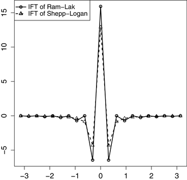
. For nonzero even integers n , (8.13) simplifies to . When n is odd, the value is given by . Figure 8.1 provides a comparison of the discrete inverse Fourier transforms of the Ram–Lak and Shepp–Logan low-pass filters, using L = 10 and sampling the inverse Fourier transforms at the Nyquist distance π∕10. Fig. 8.1
Comparison of the discrete inverse Fourier transforms of the Shepp–Logan and Ram–Lak low-pass filters, from values sampled at the Nyquist distance π∕L , with L = 10 .
Example with R 8.5.
In the preceding examples, we computed the discrete inverse Fourier Transforms for the Shepp–Logan and Ram–Lak low-pass filters. It is easy enough to record this in R. Then we evaluate at a set of points and draw the plot, like so.
L=10.0 #sets the window
xval=(pi/L)*(-L:L) #sample at Nyquist dist.
##Inverse Fourier transform of the Ram-Lak filter:
IFRL=-function(n){
ifelse(n==0,(0.5)*L^2/pi,
((0.5)*L^2/pi)*(2*sin(pi*n)/(pi*n)-(sin(pi*n/2)/(pi*n/2))
^2))}
yval1=IFRL(-L:L)
##Inverse Fourier transform of the Shepp-Logan (sinc)
filter:
IFSL=function(n){
(4*L^2/pi^3)*(1/(1-4*n^2))}
yval2=IFSL(-L:L)
### plot ##
plot(xval,yval1,pch=1,lwd=2,xlab=””,ylab=””)
lines(xval,yval1,lwd=2,lty=1,add=T)
points(xval,yval2,pch=2)
lines(xval,yval2,lwd=2,lty=2)
8.4 Discrete Radon transform
In the context of a CT scan, the X-ray machine does not assess the attenuation along every line  . Instead, in the model we have been using, the Radon transform is sampled for a finite number of angles θ between 0 and π and, at each of these angles, for some finite number of values of t . Both the angles and the t values are evenly spaced. So, in this model, the X-ray sources rotate by a fixed angle from one set of readings to the next and, within each setting, the individual X-ray beams are evenly spaced. This is called the parallel beam geometry.
. Instead, in the model we have been using, the Radon transform is sampled for a finite number of angles θ between 0 and π and, at each of these angles, for some finite number of values of t . Both the angles and the t values are evenly spaced. So, in this model, the X-ray sources rotate by a fixed angle from one set of readings to the next and, within each setting, the individual X-ray beams are evenly spaced. This is called the parallel beam geometry. If the machine takes scans at N different angles, incremented by  , then the specific values of θ that occur are
 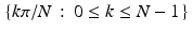 . We are assuming that the beams at each angle form a set of parallel lines. The spacing between these beams, say τ , is called the sample spacing. For instance, suppose there are 2 ⋅ M + 1 parallel X-ray beams at each angle. With the object to be scanned centered at the origin, the corresponding values of t are {j ⋅ τ : −M ≤ j ≤ M} . (The specific values of M and τ essentially depend on the design of the machine itself and on the sizes of the objects the machine is designed to scan.) Thus, the continuous Radon transform
  is replaced by the discrete function
  defined, for − M ≤ j ≤ M and 0 ≤ k ≤ (N − 1) , by
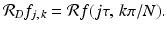
, then the specific values of θ that occur are . We are assuming that the beams at each angle form a set of parallel lines. The spacing between these beams, say τ , is called the sample spacing. For instance, suppose there are 2 ⋅ M + 1 parallel X-ray beams at each angle. With the object to be scanned centered at the origin, the corresponding values of t are {j ⋅ τ : −M ≤ j ≤ M} . (The specific values of M and τ essentially depend on the design of the machine itself and on the sizes of the objects the machine is designed to scan.) Thus, the continuous Radon transform is replaced by the discrete function defined, for − M ≤ j ≤ M and 0 ≤ k ≤ (N − 1) , by(8.14)
Example with R 8.6.
In Examples 2.13 and 2.15, in Chapter 2, we used R to compute and display sinograms for a variety of phantoms. Since R is a discrete programming environment by design, we were actually computing the discrete Radon transform of each phantom. Indeed, our first step was to define the sets of values for both t and θ to be included in the scan. Then we created a vector whose entries were the values  for all j and k .
for all j and k .To implement formula (8.2), we must now decide what we mean by the convolution of two functions for which we have only sampled values. At the same time, we will adopt some rules and conventions for dealing with discretely defined functions in general.
8.5 Discrete functions and convolution
A discrete function of one variable is a mapping from the integers into the set of real or complex numbers. In other words, a discrete function g may be thought of as a two-way infinite list, or sequence, of real or complex numbers 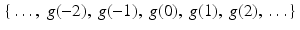 . Because of this connection to sequences, we will often write g n instead of g(n) to designate the value of a discrete function g at the integer n.
. Because of this connection to sequences, we will often write g n instead of g(n) to designate the value of a discrete function g at the integer n.Remark 8.7.
Most of the discrete functions considered here arise by taking a continuous function, say g , and evaluating it at a discrete set of values, say  . The subscript notation allows us to denote the discrete function also by g, with
  . The definition of the discrete Radon transform, in (8.14), is an example of this notation.
. The subscript notation allows us to denote the discrete function also by g, with . The definition of the discrete Radon transform, in (8.14), is an example of this notation.Definition 8.8.
In analogy with the integral that defines continuous convolution, the discrete convolution of two discrete functions f and g , denoted by  , is defined by
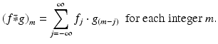
, is defined by(8.15)
As with infinite integrals, there is the issue, which we evade for the time being, of whether this sum converges.
Proposition 8.9.
A few properties of discrete convolution are
(i)
 ,
,
, (ii)
 , and
, and
, and (iii)
 ,
,
, for suitable functions f , g , and h , and for any constant α .
In practice, we typically know the values of a function f only at a finite set of points, say  , where N is the total number of points at which f has been computed and τ is the sample spacing. For simplicity, let f k = f(k τ) for each k between 0 and (N − 1) and use the set of values
  to represent f as a discrete function. There are two useful ways to extend this sequence to one that is defined for all integers. The simplest approach is just to pad the sequence with zeros by setting f k = 0 whenever k is not between 0 and N − 1. Another intriguing and useful idea is to extend the sequence to be periodic with period N. Specifically, for any given integer m, there is a unique integer n such that
  . We define
  . Thus,
  ,
,  ,
,  , and so on. This defines the discrete function f = { f k } as a periodic function on the set of all integers. We will refer to such a function as an N-periodic discrete function.
, where N is the total number of points at which f has been computed and τ is the sample spacing. For simplicity, let f k = f(k τ) for each k between 0 and (N − 1) and use the set of values to represent f as a discrete function. There are two useful ways to extend this sequence to one that is defined for all integers. The simplest approach is just to pad the sequence with zeros by setting f k = 0 whenever k is not between 0 and N − 1. Another intriguing and useful idea is to extend the sequence to be periodic with period N. Specifically, for any given integer m, there is a unique integer n such that . We define . Thus, , , , and so on. This defines the discrete function f = { f k } as a periodic function on the set of all integers. We will refer to such a function as an N-periodic discrete function. Definition 8.10.
For two N-periodic discrete functions  and
and  , the discrete convolution, denoted as before by
  , is defined by
and , the discrete convolution, denoted as before by , is defined by(8.16)
This is obviously similar to Definition 8.8 except that the sum extends only over one full period rather than the full set of integers. Notice that when m and j satisfy 0 ≤ m, j ≤ (N − 1) , then the difference (m − j) satisfies  . The periodicity of the discrete functions enables us to assign values to the discrete convolution function at points outside the range 0 to (N − 1) , so that
  also has period N .
. The periodicity of the discrete functions enables us to assign values to the discrete convolution function at points outside the range 0 to (N − 1) , so that also has period N .The two versions of discrete convolution in (8.15) and (8.16) can be reconciled if one of the two functions has only finitely many nonzero values.
Proposition 8.11.
Let f and g be two-way infinite discrete functions and suppose there is some natural number K such that g k = 0 whenever k < 0 or k ≥ K . Let M be an integer satisfying M ≥ K − 1 and let  and
and  be the (2M + 1)-periodic discrete functions defined by
  and
and  for − M ≤ m ≤ M . Then, for all m satisfying 0 ≤ m ≤ K − 1,
and be the (2M + 1)-periodic discrete functions defined by and for − M ≤ m ≤ M . Then, for all m satisfying 0 ≤ m ≤ K − 1,(8.17)
Proof.
Let f , g , K , M ,  , and
, and  be as stated. For each pair of integers m and j satisfying 0 ≤ m, j ≤ K − 1 , it follows that
 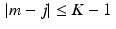 . Thus, since M ≥ K − 1 , we get that
 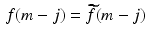 . Now fix a value of m with 0 ≤ m ≤ K − 1 . From the definition (8.15) and the properties of
  , we have
, and be as stated. For each pair of integers m and j satisfying 0 ≤ m, j ≤ K − 1 , it follows that . Thus, since M ≥ K − 1 , we get that . Now fix a value of m with 0 ≤ m ≤ K − 1 . From the definition (8.15) and the properties of , we haveWhat is really going on in this proposition? Well, there are a few worries when it comes to using periodic discrete functions. One concern is that it may not be clear what the appropriate period is. So, we might sample a finite set of values of a continuous periodic function, but the values we compute might not correspond to a full period. Then, when we extend the data to form a discrete periodic function, we have the wrong one. Or, the function whose values we have sampled might not be periodic at all. Then we ought not to use a periodic discrete function to model it. The proposition offers a remedy that is known as zero padding: we can take a finite set of values of a function ( g ) and, by padding the sequence of values with a lot of zeros, form a periodic discrete function ( ) in such a way that the periodic discrete convolution gives the same value as the true discrete convolution, at least at the points where the value has been sampled.
) in such a way that the periodic discrete convolution gives the same value as the true discrete convolution, at least at the points where the value has been sampled.For an illustration of the benefits of zero padding, consider the function  defined, as before, by
 Suppose we sample
  at two points
  and x = 0 and, so generate the 2-periodic discrete function f with
  . For the periodic discrete convolution
  , we get
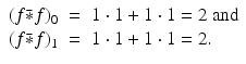 Now pad the function f with a couple of zeros to get the 4-periodic function
 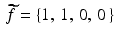 . (We could also think of this as sampling the function
  at the x values
  , 0, 1∕2, and 1.) Then we get
 Instead of accurately representing
  , the function f acts like a constant, and so
  is constant, too. But
  does a better job of representing
  , and the convolution
  is a discrete version of the function
  , for − 1 ≤ x < 1, sampled at the x values
  , 0, 1∕2, and 1.
defined, as before, by at two points and x = 0 and, so generate the 2-periodic discrete function f with . For the periodic discrete convolution , we get. (We could also think of this as sampling the function at the x values , 0, 1∕2, and 1.) Then we get, the function f acts like a constant, and so is constant, too. But does a better job of representing , and the convolution is a discrete version of the function , for − 1 ≤ x < 1, sampled at the x values , 0, 1∕2, and 1.Importantly, Proposition 8.11 applies to the discrete convolution of a sampled version of the band-limited function  , where A is a low-pass filter, and the discrete (sampled) Radon transform
  , where f is the attenuation function we wish to reconstruct. Since the scanned object is finite in size, we can set
  whenever | j | is sufficiently large. Thus, with enough zero padding, the discrete Radon transform (8.14) can be extended to be periodic in the radial variable ( j τ ), and (8.17) shows how to compute the desired discrete convolution.
, where A is a low-pass filter, and the discrete (sampled) Radon transform , where f is the attenuation function we wish to reconstruct. Since the scanned object is finite in size, we can set whenever | j | is sufficiently large. Thus, with enough zero padding, the discrete Radon transform (8.14) can be extended to be periodic in the radial variable ( j τ ), and (8.17) shows how to compute the desired discrete convolution.For discrete functions defined using polar coordinates, the discrete convolution is carried out in the radial variable only. In particular, for a given filter A , we compute the discrete convolution of the sampled inverse Fourier transform of A with the discrete Radon transform of f as
(8.18)
Example with R 8.12.
In Example 7.15, in Chapter 7, we applied the convolve procedure in R to compute the back projection of the Radon transform of a function. As mentioned there, this procedure is inherently a discrete convolution, provided one remembers to flip one of the two discrete functions involved. The option type =”open” that we used in that example applies zero padding to the sequences before computing the convolution. In the next section, we will apply convolve as one step in the implementation of the filtered back projection formula (8.2).
8.6 Discrete Fourier transform
For a continuous function f , the Fourier transform is defined by
 for every real number ω . For a discrete analogue to this, we consider an N-periodic discrete function f . Replacing the integral in the Fourier transform by a sum and summing over one full period of f yields the expression
 Now take ω to have the form
  . Then, for each choice of k , we get
  . This is a periodic function with period N in the j variable, just as f k has period N in the k variable. In this way, the Fourier transform of the discrete function f is also a discrete function, defined for ω j , with
 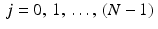 , and extended by periodicity to every integer.
. Then, for each choice of k , we get . This is a periodic function with period N in the j variable, just as f k has period N in the k variable. In this way, the Fourier transform of the discrete function f is also a discrete function, defined for ω j , with , and extended by periodicity to every integer.Definition 8.13.
The discrete Fourier transform , denoted by  , transforms an N-periodic discrete function f into another N-periodic discrete function
  defined by
For other integer values of j , the value of  is defined by the periodicity requirement.
, transforms an N-periodic discrete function f into another N-periodic discrete function defined by(8.19)
is defined by the periodicity requirement.Remark 8.14.
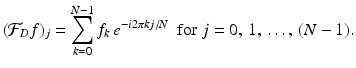
In the summation (8.19), we can replace the range 0 ≤ k ≤ (N − 1) by any string of the form 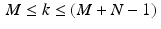 , where M is an integer. This is due to the periodicity of the discrete function f .
, where M is an integer. This is due to the periodicity of the discrete function f .Example 8.15.
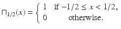
Fix a natural number M and set
 Now let N > 2M and think of f as being an N -periodic discrete function. (Thus, f consists of a string of 1s possibly padded with some 0 s.) We might think of f as a discrete sampling of the characteristic function of a finite interval. The continuous Fourier transform of a characteristic function is a function of the form asin(bx)∕x .
In the discrete setting, use the periodicity of f to compute, for each  ,
,
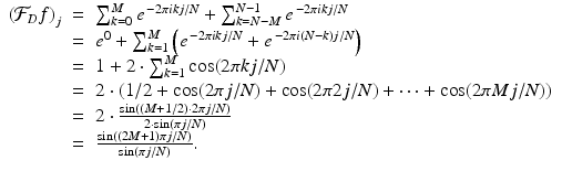 We have used the identity
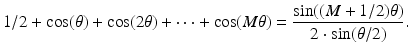
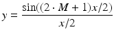
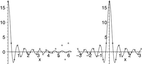
Figure 8.2 shows a comparison, with M = 8 and N = 20, of the graph of
 with the set of points
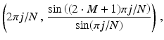 where the point (0, (2 ⋅ M + 1)) corresponds to j = 0. The diagram on the left shows the situation for 0 ≤ x ≤ 2π and
  . While the curve continues its decay, the points representing the discrete Fourier transform reveal the N-periodic behavior. In the diagram on the right, the interval is −π ≤ x ≤ π, corresponding to
  . In comparing the two diagrams, we can see how the N-periodic behavior of the discrete Fourier transform works.
,(8.20)
. While the curve continues its decay, the points representing the discrete Fourier transform reveal the N-periodic behavior. In the diagram on the right, the interval is −π ≤ x ≤ π, corresponding to . In comparing the two diagrams, we can see how the N-periodic behavior of the discrete Fourier transform works.Fig. 8.2
Continuous and discrete Fourier transforms of a square wave. Zero padding has been used in the sampling of the square wave. The wrap around in the second picture illustrates the N-periodic behavior of the discrete transform.
Where there is a discrete Fourier transform, there must also be an inverse transform. Indeed, the formula (8.2) demands it. To this end, we have the following.
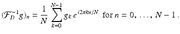
Definition 8.16.
For an N-periodic discrete function g , the discrete inverse Fourier transform of g is the N-periodic function defined by