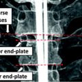
Monitoring of Bone Formation in Ankylosing Spondylitis Using Computed Tomography

Fig. 1

Example of syndesmophyte growth from baseline (BL) to year 1 (Y1) visible on CT reformations but not on radiographs

To overcome the limitations of radiographic methods, we designed a computer algorithm that quantitatively measures syndesmophyte volumes in the 3D space of CT scans [32, 33]. The algorithm is described in the following section. In Sect. 3, we investigate its accuracy and precision. Results of a 2-year longitudinal study are presented in Sect. 4. We review the future challenges of the new method in Sect. 5 before concluding in Sect. 6.

2 The Algorithm

The complete algorithm, summarized in Fig. 2, has of three main parts. First, vertebral bodies are segmented using a 3D multi-stage level set method. Triangular meshes representing the surfaces of the segmentations are made [34]. The 3D surfaces shown in Fig. 2 are triangular meshes obtained from our segmentation results. The vertebral surfaces of corresponding vertebrae are then registered. The purpose of the registration is to extract the syndesmophytes of both vertebrae using the same reference level. Syndesmophytes are cut from the vertebral body using the end plate’s ridgeline as the reference level.

Fig. 2

Overview of the complete algorithm

2.1 Segmentation of the Vertebral Bodies

Many image processing segmentation techniques have previously been applied to the extraction of vertebral bodies in CT [35–42]. For our algorithm, we chose to use level sets for their flexibility [43]. Flexibility is essential in our application as syndesmophytes can deform the normal vertebral shape in unexpected ways. Level sets are evolving contours or surfaces that can expand, contract, and even split or merge. For the purpose of segmentation they are designed to deform so as to match an object of interest. Many different types of level set exist, depending on the image features chosen to guide the segmentation. For our particular purpose, we selected two level sets based on edge features: the geodesic active contour (GAC) [44] and what we call for convenience the classical level set (CLS) [43]. The GAC evolves according to the equation [44]:

$\frac{d\psi }{dt} = \alpha g\left( {\vec{x}} \right)c\left| {\nabla \psi } \right| + \beta g\left( {\vec{x}} \right)\kappa \left| {\nabla \psi } \right| + \gamma \nabla g\left( {\vec{x}} \right)\nabla \psi$

(1)

Contours encoded as the zero level set of a distance function $\psi \left( {\vec{x},t} \right)$ : points that verify $\psi \left( {\vec{x},t} \right) = 0$ form the contour. The three terms on the right-hand side of the equation respectively control the expansion or contraction of the contour (velocity c), the smoothness of the contour using the mean curvature $\kappa$ and the adherence of the contour to the boundary of the object to be segmented. The last term, often called advection term, is specific to the GAC and is responsible for its robustness to gaps in an object’s boundary. The parameters $\alpha$ , $\beta$ and $\gamma$ allow the user to weight the importance of each term. The spatial function $g\left( {\vec{x}} \right)$ , often called speed function, is derived from the images to be segmented and contains information about the objects’ boundaries. The design of the speed function is crucial for the success of the segmentation. Depending on the specific needs of the application, information on the object’s boundary can be based on image gradient, Laplacian or any other relevant feature. The CLS is equivalent to the GAC without the advection term. The omission of the advection term makes the CLS more flexible.

A vertebral body is composed of trabecular bone surrounded by denser cortical bone. Syndesmophytes are made of cortical bone (Fig. 1). To capture those different components, we adopted a multistage strategy in which successive level sets segment the trabecular and cortical bone. Our algorithm is also multiscale. It was originally uniscale [45] but we found that multiscaling made the segmentation not only faster but also more robust and accurate. Our multiscale, multistage, 3D segmentation algorithm is summarized in the flowchart in Fig. 3. We first linearly subsample our data (step 1). Then the original algorithm is applied to the obtained half-scale volume. The preprocessing (described below) determines the parameters of the sigmoid used to compute the speed function of the first GAC (step 2.1). The first GAC roughly segments the interior of the vertebra (step 2.2). Its seed is the result of a fast marching (FM) stage starting from a seed point roughly placed by the user in the center of the vertebral body and lasting 20 iterations. The second level set, also a GAC, refines this segmentation using a Laplacian convolution of the image as the speed function (step 2.3). The third level set, a CLS, segments the cortical bone (step 2.4). A postprocessing step fills some remaining holes using a dilation followed by an erosion (step 2.5). The resulting segmentation is then super-sampled back to full scale (step 3) and refined using a CLS (step 4). A last hole-filling postprocessing is performed (step 5).

Fig. 3

Flowchart of the algorithm for segmenting vertebral bodies

The speed function $g\left( {\vec{x}} \right)$ should ideally have values close to 1 where there are no boundaries (so that the level set can expand rapidly) and values close to 0 where boundaries are present (so that the level set stops). This can be achieved for instance by writing [46]:

$g\left( {\vec{x}} \right) = 1 - \frac{1}{{1 + \exp \left( { - \frac{I - \xi }{\eta }} \right)}}$

(2)

where I is the gradient magnitude of the grey level image at voxel $\vec{x}$ . The two parameters $\xi$ and $\eta$ are typically computed using the equations [46]:

$\eta = \frac{{K_{1} - K_{2} }}{6}\quad \quad \xi = \frac{{K_{1} + K_{2} }}{2}$

(3)

where K ₁ is the minimum gradient magnitude value along the object’s boundary and K ₂ the average gradient magnitude inside the object where the level set is initialized. Those definitions ensure that the level set advances over internal gradients but stops at the minimum gradient along the boundary, as Eq. (2) maps gradients values up to K ₂ to approximately 1 and gradient values equal or larger than K ₁ to approximately 0. K ₂ can be evaluated as the mean gradient magnitude inside a neighborhood around the seed placed by the user in the center of the vertebral body. K ₁ can be determined by a search algorithm. Along lines originating from the center of the vertebral body, the maximal gradient magnitude is considered as belonging to the object’s boundary and is recorded. The mean of the 10 % lowest recorded values constitutes our estimate for K ₁ [32]. 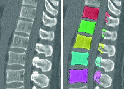The optimal values for parameters $\alpha$ , $\beta$ and $\gamma$ were determined experimentally [32]. Figure 4 shows an example of segmentation obtained by the algorithm.

Fig. 4

Example of vertebral body segmentation (original image on the left, segmentation results on the right)

2.2 Segmentation of the Vertebral Body Ridgelines

The segmentation of vertebral body ridgelines is a preliminary step to both the registration stage (Sect. 2.3) and the syndesmophyte extraction stage (Sect. 2.4). The vertebral body ridgelines provide the landmarks that aid the registration process and the reference level from which syndesmophytes are cut. We extract the ridgelines from the triangular meshes representing the surfaces of the vertebrae using the same level set as Eq. (1), but transposed from the Cartesian domain of rectangular grids to the domain of a surface mesh. While in the usual image grids of CT scans the relevant features are grey level gradients, on a surface mesh, the useful features are curvature measures (the vertebral body surface is more curved at the ridgelines than on the end plates). The curvature measure we used is curvedness (C) [47]:

$C = \sqrt {\frac{{\kappa_{1}^{2} + \kappa_{2}^{2} }}{2}}$

(4)

where $\kappa_{1}$ and $\kappa_{2}$ are the principal curvatures. Curvedness is a local measure that can be computed at each vertex on the mesh. The larger C is, the more curved the local surface is. The speed function, constructed using Eqs. 2 and 3 but with curvedness replacing grey level gradients, ensures that the level set contour expands in the center of the end plates (low curvedness) and stops at the ridgelines (high curvedness) [32].

The level set evolution equation (Eq. 1) can be implemented on a mesh with two important adjustments relative to level sets in rectangular grids: (1) Gradients and curvatures have to be computed in local coordinate systems defined around each vertex as small enough neighborhoods can reasonably be considered planar. (2) Gradients and curvatures have to be computed using least square estimation methods rather than finite differences [32].

We use the following definitions and notations for level sets on mesh. A function $f\left( V \right)$ defined on a mesh associates to each vertex $$V$$

the quantity $f\left( V \right)$ . A vertex $$V$$

is defined by its three coordinates (x, y, z) which can be relative to a global or a local orthonormal frame. $$V$$

can therefore also be seen as a vector. By immediate neighbor of vertex $$V$$

, we mean a vertex linked to $$V$$

by an edge. The 1-ring neighborhood of $$V$$

is the set of immediate neighbors of $$V$$

. The 2-ring neighborhood of $$V$$

consists of its 1-ring neighborhood and all the immediate neighbors of the vertices in the 1-ring neighborhood. The process can be iterated. Thus, the n-ring neighborhood of $$V$$

is comprised of its (n − 1)-ring neighborhood and all the immediate neighbors of the vertices in the (n − 1)-ring neighborhood.

To implement Eq. 1, the gradients of the distance function $\psi$ and the speed function $$g$$

have to be evaluated. We do this locally on the mesh in a 1-ring neighborhood around each vertex. The components of $\nabla f\left( V \right)$ the gradient of any function $$f$$

at vertex

can be evaluated by minimizing:

$E = \sum\limits_{i = 1}^{N} {\left( {\nabla f\left( V \right) \cdot \vec{n}_{i} - \nabla f\left( V \right)_{i} } \right)^{2} }$

(5)

The summation is over the N immediate neighbors of $$V$$

. The ith neighbor $V_{i}$ of $$V$$

defines the unit directional vector $\vec{n}_{i}$ :

$\vec{n}_{i} = \frac{{V_{i} - V}}{{\left| {V_{i} - V} \right|}}$

(6)

The quantity $\nabla f\left( V \right)_{i}$ is the finite difference of function $$f$$

in the direction of the ith neighbor $V_{i}$ :

$\nabla f\left( V \right)_{i} = \frac{{f\left( {V_{i} } \right) - f\left( V \right)}}{{\left| {V_{i} - V} \right|}}$

(7)

The vector components in Eqs. (5)–(7) are relative to local orthonormal frames defined at each vertex $$V$$

. The gradients $\nabla \psi$ and $\nabla g$ in Eq. (1) are computed using Eqs. (5)–(7). $\nabla \psi$ is then used to compute the mean curvature $\kappa$ .

The gradient $\nabla \psi$ is used to form two functions on the mesh: $\psi_{x} \left( V \right)$ and $\psi_{y} \left( V \right)$ , which respectively associate the x and y components of $\nabla \psi$ to each vertex $$V$$

. We can then evaluate the gradients of $\psi_{x} \left( V \right)$ and $\psi_{y} \left( V \right)$ using Eqs. (5)–(7), which in turn yields $\psi_{xx}$ , $\psi_{xy}$ and $\psi_{yy}$ . Those are the quantities necessary to compute the mean curvature $\kappa$ of the distance function $\psi$ :

$\kappa = \frac{{\psi_{xx} \psi_{y}^{2} - 2\psi_{x} \psi_{y} \psi_{xy} + \psi_{yy} \psi_{x}^{2} }}{{\left( {\psi_{x}^{2} + \psi_{y}^{2} } \right)^{\frac{3}{2}} }}$

(8)

The seeding for the mesh level set is also derived from the user placed seed for the vertebral body segmentation. From that seed (roughly in the center of the vertebral body), a vertical line cuts the upper and lower end plates in two points. Those points are used as the seeds for the mesh level sets on the upper and lower end plates. An alternative seeding technique without user input and that relies on the clustering of vertices with low curvedness has recently been proposed [48]. Figure 5 shows an example of contour evolution on the upper end plate of a vertebra. Figure 6 shows several examples of final segmentation results.

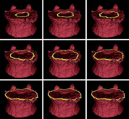
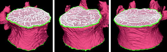
Fig. 5

Example of level set evolution on a mesh

Fig. 6

Examples of end plate (white) and ridgeline (green) segmentation

2.3 Vertebral Body Registration

Ideally, ridgelines detected on different scans of the same vertebra should be located at identical positions at the junction where the syndesmophytes merge with the end plates. In reality, those positions can be subject to variations, especially for syndesmophytes that do not grow at a right angle in respect to the end plate but laterally and merge with the end plate in a smooth gradual junction. In such cases, the curvature at the junction can be low and the level set might stop at the syndesmophyte’s base or slightly leak into the syndesmophyte depending on differing image resolution, sharpness or noise. Figure 7 shows such a discrepancy between baseline and year 1 ridgelines, with a small leak at year 1 (red arrow). Bone above the ridgeline will be labeled as syndesmophyte. If the syndesmophytes at baseline and year 1 were cut from their respective ridgelines, the leak in the year 1 syndesmophyte would cause a deficit in volume compared to baseline. This difference would not be due to real syndesmophyte change. Because real growth may be small, it is important to reduce the error coming from ridgeline discrepancies. We use registration to correct such inconsistencies. Registration aligns the vertebral bodies of scans (middle of Fig. 2). Once the vertebral bodies are registered, either of the two ridgelines can be used. The important point is to use only one of the ridgelines so that the same syndesmophyte is cut from the exactly the same level on two scans.

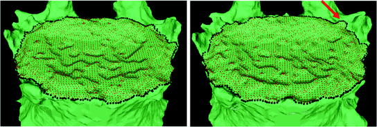
Fig. 7

End plate (red) and ridgeline (black) segmentation at baseline (left) and year 1 (right)

We used the iterative closest point (ICP) algorithm to register the surfaces of the vertebrae segmented at baseline and year 1. Given 2 sets of points, the ICP algorithm finds the rigid transformation that minimizes the mean square distance between them [49–51]. We added landmark matching to address the problem of entrapment in local minima. Our ICP algorithm is performed successively on the ridgelines, end plates and the complete surface, the result of each stage serving as the initialization for the following stage [52]. Figure 8 shows some examples of registration results.

Fig. 8

Two examples of vertebral surface registration

2.4 Syndesmophyte Segmentation

Once corresponding pairs of vertebrae are registered, syndesmophytes can be cut from the vertebral bodies using the ridgeline of the baseline vertebra (using the year 1 or 2 ridgelines is also possible). The algorithm identifies syndesmophytes in each IDS unit. The cutting algorithm marks as syndesmophyte bone voxels lying between the two end plates that bound each IDS. Because of the high precision required by our application, we found it necessary to operate this cutting with subvoxel accuracy. We also address the problem of differing degrees of smoothness in the reconstructions and partial volume effect, and refine the segmentation of syndesmophytes [33].

2.4.1 Syndesmophyte Cutting

Each IDS is bounded by the lower end plate of the superior vertebra, that we note EP1, and the upper end plate of the inferior vertebra, noted EP2. The corresponding ridgelines are respectively noted RL1 and RL2. The cutting algorithm marks as syndesmophyte those previously segmented voxels that are between those 2 end plates. Each candidate voxel is considered in relation to the local ridgelines. If it is below the local level of EP 1/RL1 and above the local level of EP2/RL2 it is marked as syndesmophyte.

However the representation of a continuous space by discrete voxels can introduce inaccuracies in this algorithm. In the first version of our algorithm, a whole voxel was considered either totally above or below the local ridgeline level [32]. However, in reality, most voxels close to the ridgeline level are neither completely above nor completely below that level. Rather, part of the voxel is above while the other part is below. The following algorithm achieves syndesmophyte cutting with subvoxel accuracy. We show how to determine the proportion of a voxel above the local level of EP2/RL2. Determining the proportion of a voxel below the local level of EP1/RL1 is straightforwardly similar.

First we extract the normal to the end plate EP2, $\vec{N}$ , using a least square estimate method [32]. Let V be a voxel under consideration. We determine the local ridgeline/end plate level in the following way. The point of RL2 closest to V is found. Neighboring points of EP2/RL2 are averaged to form the point $R_{V}$ , which, as an average, is an estimate more robust to noise. $\vec{N}$ and $R_{V}$ define a plane P (orthogonal to $\vec{N}$ and containing $R_{V}$ ), that can be used to cut syndesmophyte from vertebral body. We now determine the position of V relative to this plane. V is a rectangle defined by 8 vertices $V_{i}$ with i $\in \{1,\ldots, 8 \}.$ The sign of the scalar product:

$s\left( {V_{i} } \right) = sign(\overrightarrow {{R_{V} V_{i} }} \cdot \vec{N})$