Fig. 1
Illustration of beamline passage through multiple tissue layers and resultant superposed anatomic structures. Images from a radiographic series of the lumbar spine a frontal view, b lateral view, c coned down lateral view. Bowel loops most prominently over-project the spine on the frontal view on the image, due to photon passage through gas filled hollow viscera. Lateral and coned down lateral views demonstrate photon passage through (at different levels) and over-projection of the spine by the lungs, bowel loops, diaphragm, and internal organs (liver and spleen)
Fig. 2
Tissue density variation as manifested on radiographs. Lateral cervical spine radiograph of a 25 year old male, demonstrating examples of pixel intensity correlation with tissue density, or X-ray beam attenuation. From lesser to greater density: a air, b fatty tissue, c muscle, d bone, e metallic dental hardware
In areas where no significant different in density difference exists between adjacent normal tissue structures or between normal tissue and pathology, these structure may be not be confidently distinguishable as unique entities, and so may necessitate alternative modalities of visualization. Additionally, since three-dimensional objects are collapsed into two-dimensional data by the imaging process whereby the beam photons pass through numerous anatomic structures on their way to the detector plate, many internal structures will be superimposed on one another in the radiograph. Again, deconvolution of these objects into individually identifiable structures may necessitate alternative modalities of visualization such as cross sectional imaging. Radiographs, which are incomplete data sets, typically allow for a limited number of inferences to be drawn. Multiple orthogonal perspective views of a body structure may be taken as part of a radiographic series, increasing the information content regarding a particular structure, decreasing the level of data degeneracy and so increasing the diagnostic usefulness.
From a clinical medical perspective, radiographs commonly find use as general screening examinations for the spine, as well as for postsurgical follow-up of spinal procedures, as in Fig. 3. Relative drawbacks for radiographic imaging include lower sensitivity for certain classes of subtle pathology such as subtle fractures, low contrast in soft tissues, and patient radiation exposure.
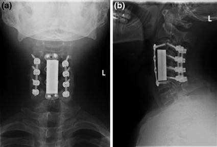
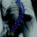
Fig. 3
Post-surgical follow up of spinal fixation procedure on a radiograph. Frontal and lateral view radiographic follow up series of spinal fixation, in a 25 year old male with history of cervical spine fracture. The patient is status-post multilevel cervical vertebral corpectomy, with anterior and posterior instrumented fusion from C3 to C6, and with integrated vertebral body strut spacer placement. Follow-up radiographic series allow for assessment of spinal alignment, as well as for inspection for hardware fracture and loosening
3 Computed Tomography
Computed tomography (CT) is a sophisticated scanning technique for creating cross sectional volumetric X-ray images of body anatomy, which are, in effect, maps of tissue density. As previously described, the beam creates X-rays which penetrate multiple layers of internal anatomy to detector banks within the scanner. The X-ray beam source and detectors rotate about the patient following a helical trajectory. The beamline is directed toward the patient, who has been placed in alignment with the central axis of the helix, with detectors positioned on the opposite sides of the patient. Thus, the X-ray source projects photons through the patient along a continuous angular progression radial beamline. An example of a CT scanner is shown in Fig. 4.
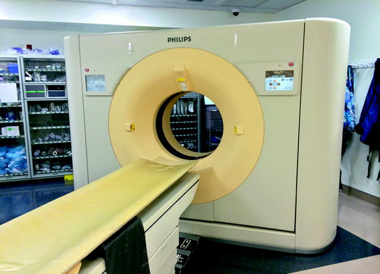
Fig. 4
Typical CT scanner unit. Patient is placed in alignment with the central axis of the helical trajectory traced by the X-ray beam source and detectors as they rotate about the patient
The extent of X-ray attenuation along the beamlines through the patient is recorded for these radial trajectories, after which complex algorithms for data reconstruction are used to separate structures along the beamlines and construct an X-ray attenuation map of the internal elements of the patient’s anatomy [3]. A volume source data set is thus derived from the patient, a three-dimensional entity, as an effective volume map of tissue density. This data is then partitioned into two-dimensional sections, typically following standardized orthogonal body planes, and stored for review by physicians who will be involved in the patient’s diagnosis and treatment. An example of this is demonstrated in Fig. 5, with a single image from each series of a CT scan of the spine, reformatted into the standardized planes for clinical interpretation. These anatomic sections have an appearance as if the body had been cross sectioned, with each sectional surface displayed as an image. High resolution sectional images in arbitrary scan planes can be created by current generation CT scanners. However, by convention, standardized orthogonal planes, relative to anatomic positioning of the body are obtained in clinical practice, in axial, coronal, and sagittal orientation relative to the long axis of the body. Additionally, a reconstruction kernel is used in producing the reformatted images, which may have higher spatial resolution, higher noise, and increased edge definition (a “bone” kernel), or improved contrast resolution, lower noise, and decreased edge definition (a “soft tissue” kernel), examples of which are shown in Fig. 6 [1].
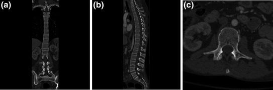
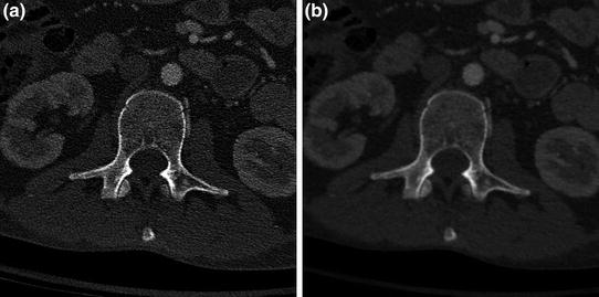
Fig. 5
CT images of the spine in standard planar reformatting. a Coronal plane image from a CT study of the spine, with the spine partially visualized on this image, due to normal kyphotic thoracic and lordotic lumbar curvature, b sagittal plane image, and c axial plane cross section at the level of the mid-abdomen. The axial field of view is kept small in this dedicated spine imaging study to increase the in-plane spatial resolution
Fig. 6
CT images of the spine demonstrating different reconstruction kernels. Axial plane images from a CT study of the spine, performed with a “bone” reconstruction kernel for the body (B70), and b “soft tissue” reconstruction kernel (B40). Note difference in edge definition and noise between images
As noted, both CT and radiographic images are produced with X-rays, and so represent surrogate maps of body organ density obtained via X-ray attenuation. Following the convention of previous generation radiographs taken on photographic film, images are mapped by grayscale, with dense structures such as bone scaled toward the white or bright end of the scale, and lower density materials scaled toward the dark end of the scale. With the invention of computed tomography, an intrinsic grayscale was created, with the scale subdivided into Hounsfield units (HU) [4, 5]. In the Hounsfield system of units, very low density structures are scaled in negative units, as in the case of air (approximately −1,000 HU) and fat (approximately −100 HU). Water is set at the standard of 0 HU, with muscle tissue scaled at approximately 40 HU and bone scaled at approximately 1,000 HU (Fig. 7).
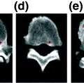
Fig. 7
Demonstration of standardized Hounsfield density units for body tissues on a CT cross section. In the CT axial cross section, measured HU in a sample ROI were a −999 within the trachea; b −105 in the fatty tissue of the axilla; c 45 in the muscle tissue of the shoulder; and d 1019 at the cortex of the scapula
On the computer monitor, Hounsfield units are scaled to pixel intensity. Medical diagnostic image display systems typically allow 10–12 bit depth, allowing the display of 1,024–4,096 shades in grayscale. Now, as the human eye can only differentiate approximately 30–40 grayscale shades, sets of restricted range brightness setting “windows” are created, centered about the tissue density of interest (Fig. 8). In materials such as bone, these windows isolate and amplify details of the anatomy of interest. The uses of CT imaging in clinical medical practice are multifold, being particularly useful for complex anatomic structures such as the spine, and for assessing certain classes of pathology such as acute fractures in non-osteopenic patients. In cases such as these, pathology on radiographic studies may be obscured or vague conferring a diagnostic advantage on CT (Fig. 9), or more complex assessment of the fracture pattern may be needed for treatment planning, again, conferring a diagnostic advantage on CT (Fig. 10). Additionally, magnetic resonance imaging may be contraindicated in certain patients, and again, CT may be helpful as a diagnostic aid. Drawbacks of CT compared to other modalities include radiation exposure to the patient, higher than for a radiograph, as well as beam hardening or streak artifact due to dense objects such as seen with orthopedic spinal fixation hardware [2].
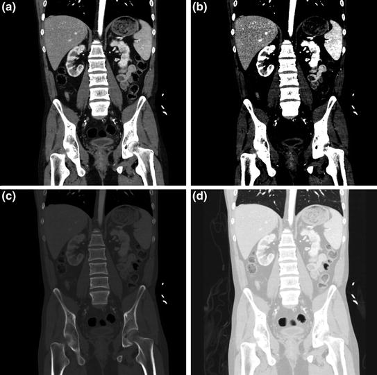
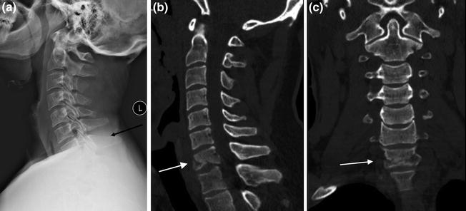
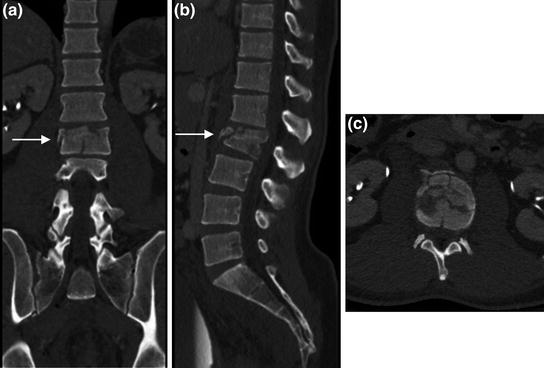
Fig. 8
Abdominal CT image set to different clinical read out windows. Coronal plane image from a CT study of the abdomen and pelvis delineating detail of multiple abdominal organs, in a general soft tissue window (here, w = 400, l = 60); b “hard contrast” soft tissue window setting (here, w = 150, l = 88) for enhancing visualization of certain abdominal organs, c bone window setting for assessment of skeletal structures (w = 2,000, l = 500); and d lung window setting (w = 1,500, l = −500) to assess air or gas containing tissues with the body, such as lungs, and hollow visci
Fig. 9
Diagnostic advantage of CT over radiographs. Patient with history of trauma and neck pain. In the lateral view radiograph of the cervical spine (a), patient’s injury is not well seen (at level of black arrow). Sagittal (b) and coronal (c) reformatted images from patient’s CT scan demonstrates comminuted fracturing of the C7 vertebra (white arrows)
Fig. 10
Spine protocol CT images. Multiplanar reformatted images from a spine protocol CT scan, in a sagittal, b colonal, and c axial planes, facilitate the extraction of detailed information regarding the vertebral fracture pattern and extent allowing a more accurate assessment for treatment planning
4 Magnetic Resonance Imaging (MRI)
Nuclear magnetic resonance (NMR) initially found widespread use in analyzing the spectral characteristics of organic compounds, based on their magnetic properties. In September of 1971, Paul Lauterbur had an idea for the application of three dimensional magnetic field gradients to produce NMR images. The first images of two spatially separate tubes containing water was published in Nature in March of 1973 [6]. This quantum advance of the invention of instruments to examine material characteristics in a spatially distributed manner, led to the design of the magnetic resonance imaging (MRI) scanner. Body tissues have intrinsic and varying magnetic properties. These characteristics are exploited in MRI to create spatially distributed images of the internal anatomy of the body, which represent cross sectional anatomic maps of the magnetic characteristics of the tissues at each spatial point in the regions being imaged.
As heuristic model for magnetic properties of tissue and the basis of MRI, consider a magnetic dipole, or for a more physically conceptual macroscopic model, a bar magnet. Recall that magnetic field lines emanate from the north pole of the bar magnet, with the south pole of the magnet acting as a sink for magnetic field lines. A characteristic quantity associated with the magnetic dipole is the magnetic moment, which is expressed with the magnetic field strength and orientation of the dipole. At the atomic level, the nuclei of atoms constituting the tissue are made up of neutrons and protons. These nucleons individually have small magnetic moments, and when they occur unpaired in the nucleus they give the nucleus a net magnetic moment. The hydrogen atom, with its unpaired proton nucleus is a constituent many of molecules in the body including water and fatty tissues, and is of keystone importance in most current clinical imaging applications.
Now, when a macroscopic “magnetic dipole” is placed into an external magnetic field, it tends toward its lowest energy state, aligning with that field (as in the conceptual macroscopic analogy of a directional compass needle). Energy must be applied to turn the compass needle (“dipole”) into a different direction, or higher energy state. Now, as we are on the atomic scale, quantum considerations come into play, and the dipole moment actually precesses about the direction of the applied field. The dipole moment of the proton nucleus will then tend to align with an applied magnetic field within quantum limits. The application of energy is achieved by the application of an electromagnetic energy in the form of a radiofrequency pulse [1]. This energy pulse is absorbed by the tissues, with resultant rotation of the magnetic moments into a higher energy state. The magnetic moments then give off energy as they relax toward lower energy states, at rates related to their local molecular environment, or tissue characteristics. Spatial variances in this relaxation rate by tissue type are detected and used as a basis for creating a spatial map of the magnetic properties of body tissue cross sections, or magnetic resonance images.
Armed with an understanding of the conceptual basis for MR imaging, we now consider the clinical application. MR imaging is performed by placing the patient into the center of a large magnet, typically structured in the overall geometry of a cylinder (Fig. 11). The magnetic polarity of the applied magnetic field is alternated at characteristic and varying frequencies and pulse settings to emphasize specific properties of the tissues. A single scan utilizing characteristic phase and frequency parameters used to emphasize specific tissue properties is termed a pulse sequence. A group of these sequences, varied in terms of the tissue planes being imaged and physical characteristics of the tissue being emphasized, forms an MRI examination.
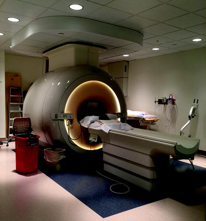
Fig. 11
MRI scanner unit. Patient is placed on a moveable table in alignment with the central axis of the magnet gantry, which then moves into the bore of the magnet during the scanning process
A multitude of MRI sequences have now been devised investigate specific tissue characteristics and pathologies. However, there is a fundamental set of sequences ubiquitous in use in medical imaging, known as T1, proton density (PD), and T2, examples of which for the spine are shown in Fig. 12 [7]. Each of these MRI sequences has benefits and drawbacks. The benefits of T1 include increased anatomic detail relative to T2 and ability to assess tissue enhancement with the administration of contrast. T2, on the other hand, is better for assessing edema and has generally shorter imaging times [8]. PD is an intermediate sequence, which seeks to combine T1 and T2 characteristics, with results which are intermediate between the two. Now, on grayscale imaging, certain tissues will show up as high signal intensity (white on the display monitor), and other as low signal intensity (black on the display monitor). On T1 imaging, fluid in the tissues presents as intermediate to low signal intensity, and fat as high signal intensity. In opposition, fluid on T2 appears as high signal and fat as high signal. Thus, in principle, one could differentiate fluid on a T2 sequence by comparison with a T1 sequence (see Fig. 12). There are exceptions to these signal intensity norms, including proteinaceous fluid in the body which can appear high signal intensity on T1.
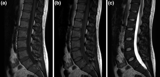
Fig. 12
Spine protocol images in varying sequence weightings. Sagittal images of the lumbar spine imaging sequences demonstrating a T1, b PD, and c T2 imaging
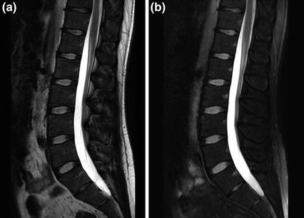
Modifications of these basic sequences have been devised to expand their range of clinical utility, including what are termed fat suppression variations. In fat suppression, a process is applied by which adipose tissue, normally high signal intensity on T1 and T2, is turned to low signal intensity. One method by which this is accomplished is called fat saturation. Fat saturation depends on the slight field-dependent variance in precession frequency between the protons of fat and water and uses a frequency selective applied excitation to nullify the fat signal intensity (Fig. 13) [8, 9]. Consider an example of the clinical usage of fat saturation on a standard T2 sequence which demonstrates high signal intensity for both fat and fluid. If the fat signal intensity is now turned low after the application of fat saturation, fluid will now be the principle residual high intensity entity left on the image, amidst an intrinsically dark background of surrounding tissues composed of shades ranging from gray to black. Thus, any structure with fluid or edema (of interest in detecting pathology) will appear prominent, facilitating the detection and characterization of pathological tissue.
 Assistance and Intervention in Spine Surgery
 Column Localization, Labeling, and Segmentation
 Aided Detection of Bone Metastases in the Thoracolumbar Spine
 Model-Based Vertebra Identification from X-Ray Image(s)
 Spine Reconstruction from Radiographs
 Segmentation, Reconstruction and Analysis of the Vertebral Body from Spinal CT


Related posts:
Assistance and Intervention in Spine Surgery
Aided Detection of Bone Metastases in the Thoracolumbar Spine
Model-Based Vertebra Identification from X-Ray Image(s)
Spine Reconstruction from Radiographs
Segmentation, Reconstruction and Analysis of the Vertebral Body from Spinal CT
Stay updated, free articles. Join our Telegram channel
Full access? Get Clinical Tree
