Fig. 1
Vertebral Body: A CT slice of vertebral body illustrates its regions: the VB region (in blue color), which is our region of interest to be segmented. Spinal processes and ribs, which should not be included in the BMD measurements, are shown as well
Fig. 2
Typical challenges for vertebrae segmentation. a Inner boundaries. b Osteophytes. c Bone degenerative disease. d Double boundary
The literature is rich with organ segmentation techniques. However, we will discuss only some of these techniques whose basics depend on shape modeling and whose application is VB segmentation. To tackle the problem of segmenting a spine bones, various approaches have been introduced. For instance, Klinder et al. [1] developed an automated model-based vertebra detection, identification and segmentation approach. Kang et al. [2] developed a 3D segmentation method for skeletal structures from CT images. Their method starts with a three dimensional region growing step using local adaptive thresholds. Then a closing of boundary discontinuities and an anatomically-oriented boundary adjustment steps are done. They presented various anatomical bony structures as applications. They evaluated their segmentation accuracy using the European Spine Phantom (ESP) [3]. In order to measure bone mineral density, Mastmeyer et al. [4] presented a hierarchical segmentation approach for the lumbar spine. They reported that it takes less than 10 min to analyze three vertebrae, which is a huge improvement compared to what is reported in [5]: 1–2 h. However, this timing is far from the real time required for clinical applications. To analyze the fracture of VBs, Roberts et al. [6] used the active appearance model. Other techniques have been developed to segment skeletal structures and can be found for instance in [7–9].
Actually, there are a huge number of segmentation techniques in the literature: simple techniques (e.g. region growing or thresholding), parametric deformable models and geometrical deformable models. However, all these methods tend to fail in the case of noise, gray level inhomogeneities, and diffused boundaries. Organs have well-constrained forms within a family of shapes. Therefore segmentation algorithms have to exploit the prior knowledge of shapes and other properties of the structures to be segmented. Leventon et al. [10] combined the shape and deformable model by attracting the level set function to the likely shapes from a training set specified by principal component analysis (PCA). To make the shape guides the segmentation process, Chen et al. [11] defined an energy functional, which basically minimizes an Euclidean distance between a given point and its shape prior. Huang et al. [12], combined registration with segmentation in an energy minimization problem. The evolving curve is registered iteratively with a shape model using the level sets. They minimized a certain function to estimate the transformation parameters.
In this chapter, we present universal and probabilistic shape based segmentation methods that are less variant to the initialization. Contribution of this chapter can be generalized as follows:
This chapter solves problems caused by noise, occlusion, and missing information of the object by integrating the prior shape information.
In this chapter, the conventional shape based segmentation results are enhanced by proposing a new probabilistic shape models and a new energy functional to be minimized. The shape variations are modelled using a probabilistic functions.
The proposed shape based segmentation method is less variant to the initialization.
To optimize the energy functional, the original ICM method, which was originally proposed by Besag [13], is extended by integrating the shape prior. With integrating the shape model to the original ICM method, possible local minimums of the energy functional are eliminated as much as possible, and enhance the results.
One of the most important contributions of this study is to offer a segmentation framework which can be suitable to the clinical works with acceptable results. If the proposed method in this study is compared most published bone segmentation methods, the large execution time is reduced effectively.
Many works are restricted to the specific regions of spine bone column as such lumbar, thoracic, and others. In this study, there is no any region restriction, and the proposed framework is processed on different regions.
The proposed framework and the new probabilistic shape model extract the spinal processes and ribs which should not be included in the bone mineral density measurements.
This work is not dependent on any identification step thanks to the new universal shape model and its embedding step.
Next section details the proposed methods.
2 Proposed Framework
In this section, we describe the proposed methods. First, the general theoretical idea of the proposed frameworks is described. Then, two pre-processing steps, the spinal cord extraction and VB separation, are described. We present three methods which differ mostly in the shape modeling and optimization parts.
2.1 Overview
In this chapter, three pieces of information (intensity, spatial interaction, and shape) are modelled to obtain the optimum segmentation. The data is assumed to have two classes: background and object regions which are represented as “b” or “0” and “o” or “1”, respectively. So, let  denotes the set of labels. In this work, the given VB’s volume, the shape model and the desired map (labeled volume) are described by a joint Markov-Gibbs random field (MGRF) model. We can define the gray level volume
  by the mapping
  and its desired map
  by the mapping
  , where
  is the set of voxels and
  is the set of gray levels. Shape information is represented by the set of distances of variability region’s voxels
  (more details explained later). Since
  and
and  are independent, a conditional distribution model of input volume, its desired map, and the shape constraints can be written by the as follows:
where  and
and  represents appearance models, and the conditional distribution
  is the shape model. Given
  and
and  , the map
  can be obtained using Bayesian maximum–a posteriori estimate as follows:
where  is the set of all possible
  , and
, and  is the log-likelihood function, which can be written as follows:

denotes the set of labels. In this work, the given VB’s volume, the shape model and the desired map (labeled volume) are described by a joint Markov-Gibbs random field (MGRF) model. We can define the gray level volume by the mapping and its desired map by the mapping , where is the set of voxels and is the set of gray levels. Shape information is represented by the set of distances of variability region’s voxels (more details explained later). Since and are independent, a conditional distribution model of input volume, its desired map, and the shape constraints can be written by the as follows:(1)
and represents appearance models, and the conditional distribution is the shape model. Given and , the map can be obtained using Bayesian maximum–a posteriori estimate as follows:(2)
is the set of all possible , and is the log-likelihood function, which can be written as follows:(3)
The parameters of the shape model  and the volume appearance models should be identified, to completely define this log-likelihood function.
and the volume appearance models should be identified, to completely define this log-likelihood function.Intensity and interaction models may not be enough to obtain optimum segmentation. To segment the VB, a new shape based methods which integrate the models of the intensity, spatial interaction, and shape prior information is proposed. The proposed method presents several advantages which can be written as: (i) the probabilistic shape model is automatically registered to the testing image, hence manual interaction is eliminated, (ii) the registration benefits from the segmented region to be used in the shape representation, and (iii) the probabilistic shape model refines the initial segmentation result using the registered variability volume.
The segmentation part has following steps: (1) initial segmentation using only intensity and spatial interaction information (this step is needed to obtain the feature correspondence between the image domain and shape model), (2) shape model registration, and (3) the final segmentation using three models.
Next section, we describe the spinal cord extraction stage as a preprocessing step.
2.2 Spine Cord Extraction
As a pre-processing step, the spinal cord is extracted using the Matched filter. This process helps to remove the spinal processes roughly; hence the shape model will be registered to the image domain easily. In the first step, the Matched filter (MF) [14, 15] is employed to detect the VB automatically. This procedure eliminates the user interaction and improves the segmentation accuracy. Let  and
and  be template and test images, respectively. To compare the two images for various possible shifts
  and
and  , one can compute the cross-correlation
  as
as
where the limits of integration are dependent on  . The Eq. (4) can also be written as
where  and
and  are the 2-D FTs of
  and
and  , respectively with
  and
and  denoting the spatial frequencies. The test image
  is filtered by
  to produce the output
  . Hence,
  is the correlation filter which is the complex conjugate of the 2-D FT of the reference image
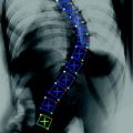
  . Figure 3a shows the reference image used in the Matched filter. Some examples of the VB detection are shown in Figs. 3b–d. The Matched filter is tested using 4,000 clinical CT images. The detection accuracy for the VB region is 97.2 %. The detection accuracy is increased to around 100 % by smoothing all detected points of a dataset in the z-axis.
and be template and test images, respectively. To compare the two images for various possible shifts and , one can compute the cross-correlation as(4)
. The Eq. (4) can also be written as(5)
and are the 2-D FTs of and , respectively with and denoting the spatial frequencies. The test image is filtered by to produce the output . Hence, is the correlation filter which is the complex conjugate of the 2-D FT of the reference image . Figure 3a shows the reference image used in the Matched filter. Some examples of the VB detection are shown in Figs. 3b–d. The Matched filter is tested using 4,000 clinical CT images. The detection accuracy for the VB region is 97.2 %. The detection accuracy is increased to around 100 % by smoothing all detected points of a dataset in the z-axis.Fig. 3
a The template used for the Matched filter. b–d A few images of automatic VB detection. The green line shows the detection of VB region
To extract the spinal processes and ribs roughly, some simple steps are followed as shown in Fig. 4. These steps are required to: (i) extract the spinal processes and ribs roughly, (ii) crop the ROI minimize the execution time. Figures 5 and 6 show different examples of this stage in the sagittal view.
Fig. 4
In the first step, the MF is run on each slice of the 3D data. The output of this process is the detected points of each CT slices as shown with the blue dot. After the center points are detected, a mask is used to refine the data to specify the region of interest (ROI). In the mask, it is accepted that  ,
,  , and
, and  . Any user can change these values. But the user should be careful to extract the spinal processes and ribs roughly. Then, another mask can be used to crop the ROI using the average center points (the red color) of all slices of 3D data.
  is accepted to capture the VB region
, , and . Any user can change these values. But the user should be careful to extract the spinal processes and ribs roughly. Then, another mask can be used to crop the ROI using the average center points (the red color) of all slices of 3D data. is accepted to capture the VB regionFig. 5
The extraction of the spinal cord on a data set (Example-1). a Sagittal view of each data. b The detected VB region. c The refined data to extract the spinal processes and ribs. d The cropped data to reduce the size of the image
Fig. 6
The extraction of the spinal cord on a data set (Example-2). a Sagittal view of each data. b The detected VB region. c The refined data to extract the spinal processes and ribs. d The cropped data to reduce the size of the image
2.3 Vertebrae Separation
This process is required in the proposed framework hence the shape model is registered to each VB in an easy way. In this process, two methods are suggested to separate each vertebrae. The first suggestion is the manual separation, and the second one is the previously proposed automatic framework [16] as shown in Fig. 7c.

Fig. 7
The separation of each VB in a data set. Two choices are given to the user: The Manual and automatic options. Each option has its own advantages and disadvantages which are described the section. a An image which has 3 adjacent VBs. b The manual separation process with 6 points selected by a user. c The automatic separation method which was proposed by Aslan et al. in [16]
The advantage of automatic separation is to eliminate user interaction(s). However, there are two disadvantages: (i) increased error, (ii) current methods in the literature have higher execution time respect to the manual methods. To give the user his own choice, two methods are described.
2.3.1 Manual
After the spinal cord, processes, and ribs are extracted roughly, we need to separate adjacent VBs in order to embed the shape model to the image domain. In the manual separation, simple manual annotations are needed to specify the cut-points of VBs. For instance, if there are three VBs in the dataset, six points are annotated on the image. In the experiments, the average execution time to separate 12 adjacent VBs is 18 s. This timing may still not be optimum one, however, with manual annotations there should not be any possible data loss. In the next section, the automated separation process, which Aslan et al. previously published in [16], is described. It should be noted that segmentation accuracy is measured when the VBs are separated manually.
2.3.2 Automatic
In this section, a 3D framework to separate vertebral bones in CT images without any user intervention [16] is used. To separate the VBs, the previously developed approach based on 4 points automatically placed on cortical shell is used. An example of separation and segmentation of a VB is shown in Fig. 8c. After the spinal cord is extracted; the approximate centerline of VB column is obtained. These seeds are placed using the relatively higher gray level intensity values of the cortex region.
Fig. 8
The separation of the VB region. a 3D view of three adjacent VB. b Automated placement of 4 seeds on cortical bone and disc. c Separation of VB shown with red color
Next, the histogram for a neighborhood around each seed is obtained. The histogram represents the number of voxels whose intensity values are above 200 Hounsfield Unit (HU). This value is obtained empirically. Vertical boundaries of a VB show higher gray level intensity than inner region of the VB and disks. Figure 9 shows histograms (the red line), and thresholds (the black line). To search vertical limits of the VB, the following adaptive threshold equation is used as follows:
![$$ TH = \mu (A) + \kappa *[{ \hbox{max} }(A) - \mu (A)], $$](/wp-content/uploads/2016/12/A312884_1_En_13_Chapter_Equ6.gif)
where  which is derived from experiments by trial-and-error, where
  represents each histogram vector with the red line as shown in Fig. 9,
  and
and  are the maximum and average values in the histogram vector.
Fig. 9
The VB separation: The green volume shows the 4 four seeds. The red lines correspond to the number of voxels whose gray level are bigger than 200 HU. The black lines correspond to the threshold written in Eq. (6)
(6)
which is derived from experiments by trial-and-error, where represents each histogram vector with the red line as shown in Fig. 9, and are the maximum and average values in the histogram vector.In the separation step,  patients which totals to
  VBs are used. The results can be classified as in [17]. There are five respective categories as described below.
patients which totals to VBs are used. The results can be classified as in [17]. There are five respective categories as described below.
Excellent: The VB is successfully separated without any misclassification. Vertical limits are correctly obtained.
Good: The VB is separated with small parts of adjacent disk or VB. Around 90 % or vertical limits are correctly obtained.
Bad: The VB is separated, however noticeable parts of it are missed. Around 70–90 % of vertical limits are correctly obtained.
Poor: Large portions of anatomical structure of VB are missed. Around 50–70 % of vertical limits are correctly obtained.
Fail: The VB is not separated due to challenges.
The proposed method produced about 85 % successful separation results, if excellent and good grades are considered. Hence, 15 % separation results were considered as fair, bad, or fail.
2.4 Segmentation Using Sign Distance-based Shape Model, Gaussian-based Intensity Model, and Symmetric Gibbs Potential-based Spatial Interaction Model
In the following subsections, we describe three proposed methods developed for the VB segmentation problem. We, first, describe each method, then show its experimental results.
The overall segmentation framework is shown in Fig. 10. The proposed framework steps are described in Algorithm 1 as follows:
Fig. 10
The general segmentation framework. (Prior to this framework, it is required to obtain the shape model). In the first phase, the spinal cord is extracted, processes, and ribs roughly using the Matched filter. Also, the data size is reduced to minimize the execution time. In the second phase, the VBs are separated with two choices: (i) manual, (ii) automatic. In the third phase, a new shape based ICM method is proposed to segment the VBs
Algorithm 1:
A(Training)): 80 training VB shapes are used to obtain the new probabilistic shape model. In this step, manually segmented VB shape which are obtained from 20 different patients and different regions (such as cervical, thoracic, and lumbar spine bone sections) are used.
B) Spinal cord extraction (Pre-processing): The Matched filter is used to detect the spinal cord. This step roughly extracts the ribs and spinal processes. Also, the data size is reduced to 120x120xZ from 512x512xZ where Z is the number of slices. This step reduces the execution time of the segmentation process. The output of this phase is used in the following steps.
C) Separation of VBs (Pre-processing): Two choices are given for the user(s)-i) manual selection of disk to obtain each VB in a datasets, ii) fully automatic VB separation using the histogram based information. It should be noted all steps of the framework are fully automated except this step.
D) Segmentation: Three models are used to segment VBs: The intensity, spatial interaction, and shape models. The following ‘While’ loop is processed for the segmentation.
While  do (
do ( : the number of slices.)
do (: the number of slices.)1)
The initial segmentation using the ICM method which integrates the intensity and spatial interaction information. Using the EM algorithm,  and
and  are estimated; and
  and
and  are estimated using the MGRF modeling. Then ICM method is used to select the optimum labeling which maximizes
  .
.
and are estimated; and and are estimated using the MGRF modeling. Then ICM method is used to select the optimum labeling which maximizes .2)
The shape model is registered to the initially segmented region.
3)
Final segmentation is carried out using the ICM which maximizes  .
.
.End While
To obtain a good intensity model, the conditional probability distribution,  , of the original image is estimated. The intensity information is modelled using the Gaussian distribution. The Gaussian function can be written as
, of the original image is estimated. The intensity information is modelled using the Gaussian distribution. The Gaussian function can be written as(7)
The parameters of distributions ( ) are estimated using the expectation-maximization (EM) method in [18, 19] where i = “0” and i = “1” represent ‘background’ and ‘object’ classes, respectively.
) are estimated using the expectation-maximization (EM) method in [18, 19] where i = “0” and i = “1” represent ‘background’ and ‘object’ classes, respectively.Spatial interaction helps correcting errors and recovering missing information in the image labeling problem [20]. Stochastic process on a random field is used to realize the image [21]. In this study, the unconditional probability distribution of the desired map (labeling),  , is obtained. To estimate
  , the Gibbs distribution is used. The Gibbs distribution takes the following form
where
is a normalizing constant called the partition function,  is a control parameter called the temperature which is assumed to be 1 unless otherwise stated, and
  is the Gibbs energy function. The energy is a sum of clique functions
  over all possible cliques
  as
as
, is obtained. To estimate , the Gibbs distribution is used. The Gibbs distribution takes the following form(8)
(9)
is a control parameter called the temperature which is assumed to be 1 unless otherwise stated, and is the Gibbs energy function. The energy is a sum of clique functions over all possible cliques as(10)
A clique is a set of sites in which all pairs of sites are neighbors. The clique potentials can be defined by
where  is the potential for type-c cliques. In this proposed method, the Potts model [22] which is similar to Derin-Elliot model [23] is used. This model uses the potentials of the Potts model describing the spatial pairwise interaction between two neighboring pixels. The MGRF with the second order (8-pixel) neighborhood depends only on the whether the nearest pairs of pixel labels are equal or not. In this method,
  is estimated using the method proposed by Ali et al. in [24].
(11)
is the potential for type-c cliques. In this proposed method, the Potts model [22] which is similar to Derin-Elliot model [23] is used. This model uses the potentials of the Potts model describing the spatial pairwise interaction between two neighboring pixels. The MGRF with the second order (8-pixel) neighborhood depends only on the whether the nearest pairs of pixel labels are equal or not. In this method, is estimated using the method proposed by Ali et al. in [24].Human anatomical structures such as spine bones, kidneys, livers, hearts, and eyes may have similar shapes. These shapes usually do not differ greatly from one individual to another. There are many works which analyze the shape variability. Cootes et al. [25] proposed effective approach using principle component analysis (PCA). Abdelmumin [26] proposed another shape based segmentation method using the Level sets algorithm. Tsai et al. [27] proposed a shape model which is obtained using a signed distance function of the training data. Eigenmodes of implicit shape representations are used to model the shape variability. Their method does not require point correspondences. Their shape model is obtained using a coefficient of each training shape. Cremers et al. [28] proposed a simultaneous kernel shape based segmentation algorithm with a dissimilarity measure and statistical shape priors. This method is validated using various image sets in which objects are tracked successfully. Most published works are theoretically valuable. However, parameter optimization of the shape priors may take high execution time if the training set is large. Also, the optimization methods used in shape registration, such as the gradient descent, takes high execution time.
For the shape definition, mathematician and statistician D.G. Kendall writes: “All the geometrical information that remains when location, scale, and rotational effects are filtered out from an object.” Hence, the shape information is modeled after the sample shapes are transformed into the reference space. Finally, the shape variability is modeled using the occurrences of the transformed shapes. In the proposed work, the vertebral body shape variability is analyzed using a probabilistic model.
In the next sections, each step is described in detail.
2.4.1 Shape Model Construction (Training)
Registration is the important method for shape-based segmentation, shape recognition, tracking, feature extraction, image measurements, and image display. Shape registration can be defined as the process of aligning two images of a scene. Image registration requires transformations, which are mappings of points from the source (reference) image to the target (sensed) image. The registration problem is formulated such that a transformation that moves a point from a given source image to another target image according to some dissimilarity measure, needs to be estimated. The dissimilarity measure can be defined according to either the curve or to the entire region enclosed by the curve. The source and target images and transformation can be defined as follows:
Source ( ): Image which is kept unchanged and is used as a reference. This image can be written as a function
  for
for  .
.
Target ( ): Image which is geometrically transformed to the source image. This image can be written as a function
  for
for  .
.
Transformation ( ): The function is used to warp the target image to take the geometry of the reference image. The transformation can be written as a function
  which is applied to a point
  in
in  to produce a transformed point which is calculated as
  . The registration error is calculated as
  for each transformed pixel.
Steps in the registration can be categorized in 5 different ways such as:
(i)
Preprocessing: Image smoothing, deblurring, edge sharpening, edge detection, and etc.
(ii)
Feature selection: Points, lines, regions and etc. from an the source and target image.
(iii)
Feature correspondence: The correspondence between two images.
(iv)
The transformation functions: Affine, rigid, projective, curved and etc.
(v)
Resampling: Transformed image should be resampled in the new image domain.
In general, there are three categories of the registration methods: rigid, affine, and elastic transformation. In literature the rigid and affine transformations are classified as global transformations and elastic transformations are as local transformation. A transformation is global if it is applied to the entire image. A transformation is local if it is a composition of two or more transformations determined on different domains (sub-images) of the image.
A rigid body transformation is the most fundamental transformation and is useful especially when correcting misalignment in the scanner. This transformation allows only translation and rotations, and preserves all lengths and angles in an image.
An affine transformation allows translation, rotation, and scaling. Some authors defined the affine transformation as the rigid transformation plus scaling. Affine transformations involving shearing (projection) are called projective transformation. An affine transformations will map lines and planes into lines and planes but does not preserve length and angles.
An elastic transformation allows local translation, rotation, and scaling, and it has more number of parameters than affine transformations. It can map straight lines into curves. An elastic registration is also called as a non-linear or curved transformation. This transformation allows different regions to be transformed independently.
2.4.2 The Registration of Training Shapes
For the training stage,  VB cross-sections (
 thoracic,
  lumbar,
  cervical) are used. These VBs are selected form
  healthy and
  with low bone mass patients. The more information about the testing CT data sets will be given in the experimental section.
VB cross-sections ( thoracic, lumbar, cervical) are used. These VBs are selected form healthy and with low bone mass patients. The more information about the testing CT data sets will be given in the experimental section.In this subsection, we overview the shape representation approach used in this work. The training set consists of VB shapes, { }, as shown in Fig. 11; with the signed distance functions {
 }. Any pixel in this shape representation is shown as
  . The registration of all training shapes is done using the similar approach described in [28] and used in [29, 30] as follows:
}, as shown in Fig. 11; with the signed distance functions { }. Any pixel in this shape representation is shown as . The registration of all training shapes is done using the similar approach described in [28] and used in [29, 30] as follows:Fig. 11
a The training VB images. In this experiment, 80 VB shapes which are obtained from 20 different patients and different regions (such as cervical, thoracic, and lumbar spine bone sections) are proposed. b The average shape of all training VB images. The darker color represents the higher object probability
1.
First, the average of the position factor ( ) and scale factor (
 ) are obtained using the following equations
![$$ \mu = \left[ {\begin{array}{*{20}c} {\mu_{x} } & {\mu_{y} } \\ \end{array} } \right]^{T} = \left[ {\begin{array}{*{20}c} {\frac{{\sum\nolimits_{i = 1}^{N} {\sum\nolimits_{\Upomega } {xH( - \phi_{i} ({\mathbf{x))}}} } }}{{\sum\nolimits_{i = 1}^{N} {\sum\nolimits_{\Upomega } {H( - \phi_{i} ({\mathbf{x))}}} } }}} & {\frac{{\sum\nolimits_{i = 1}^{N} {\sum\nolimits_{\Upomega } {yH( - \phi_{i} ({\mathbf{x))}}} } }}{{\sum\nolimits_{i = 1}^{N} {\sum\nolimits_{\Upomega } {H( - \phi_{i} ({\mathbf{x))}}} } }}} \\ \end{array} } \right]^{T} , $$](/wp-content/uploads/2016/12/A312884_1_En_13_Chapter_Equ12.gif)
![$$ \sigma = \left[ {\begin{array}{*{20}c} {\sigma_{x}^{2} } & {\sigma_{y}^{2} } \\ \end{array} } \right]^{T} = \left[ {\begin{array}{*{20}c} {\frac{{\sum\nolimits_{i = 1}^{N} {\sum\nolimits_{\Upomega } {(x - \mu_{x} )^{2} H( - \phi_{i} ({\mathbf{x))}}} } }}{{\sum\nolimits_{i = 1}^{N} {\sum\nolimits_{\Upomega } {H( - \phi_{i} ({\mathbf{x))}}} } }}} & {\frac{{\sum\nolimits_{i = 1}^{N} {\sum\nolimits_{\Upomega } {(y - \mu_{y} )^{2} H( - \phi_{i} ({\mathbf{x))}}} } }}{{\sum\nolimits_{i = 1}^{N} {\sum\nolimits_{\Upomega } {H( - \phi_{i} ({\mathbf{x))}}} } }}} \\ \end{array} } \right]^{T} , $$](/wp-content/uploads/2016/12/A312884_1_En_13_Chapter_Equ13.gif)
where  is the Heaviside step function.
) and scale factor () are obtained using the following equations(12)
(13)
is the Heaviside step function.2.
A global transformation is used to register training shapes with scale and translation parameters. The transformation has scaling,  , and translation components
  . Obtain the transformation parameters (
 ) for each training shape,
  , as
, as
![$$ {\mathbf{Tr}} = \left[ {\begin{array}{*{20}c} {t_{x} } & {t_{y} } \\ \end{array} } \right]^{T} = \left[ {\begin{array}{*{20}c} {\mu_{x} - \frac{{\sum\nolimits_{\Upomega } {xH( - \phi ({\mathbf{x))}}} }}{{\sum\nolimits_{\Upomega } {H( - \phi ({\mathbf{x))}}} }}} & {\mu_{y} - \frac{{\sum\nolimits_{\Upomega } {yH( - \phi ({\mathbf{x))}}} }}{{\sum\nolimits_{\Upomega } {H( - \phi ({\mathbf{x))}}} }}} \\ \end{array} } \right]^{T} , $$](/wp-content/uploads/2016/12/A312884_1_En_13_Chapter_Equ14.gif)
![$$ {\mathbf{S = }}\left[ { \begin{array}{*{20}l} {s_{x} } \hfill & 0 \hfill \\ 0 \hfill & {s_{y} } \hfill \\ \end{array} } \right] = \left[ {\begin{array}{*{20}c} {\frac{{\sigma_{x} }}{{\sqrt {\frac{{\sum\nolimits_{\Upomega } {(x - \mu_{x} )^{2} H( - \phi ({\mathbf{x}}))} }}{{\sum\nolimits_{\Upomega } {(H - \phi ({\mathbf{x}}))} }}} }}} & 0 & {} & {} \\ 0 & {\frac{{\sigma_{y} }}{{\sqrt {\frac{{\sum\nolimits_{\Upomega } {(y - \mu_{y} )^{2} H( - \phi ({\mathbf{x}}))} }}{{\sum\nolimits_{\Upomega } {H( - \phi ({\mathbf{x}}))} }}} }}} & {} & {} \\ \end{array} } \right]^{T} $$](/wp-content/uploads/2016/12/A312884_1_En_13_Chapter_Equ15.gif)
, and translation components . Obtain the transformation parameters () for each training shape, , as(14)
(15)
3.
The transformation will be in the form  , where
  is the transformed point of
  .
.
, where is the transformed point of .Note: In 2D case, the rotation parameter for the VB shape registration is not necessary since VB shape does not show important variation in different rotation.
2.4.3 Training stage (Obtaining Probabilistic Shape Model)
1.
Segment training images manually.
2.
Align segmented images.
3.
Generate shape variation. Intersection of training shape is accepted as an object volume. The rest of the volume is accepted as variability volume except the background region.
4.
Obtain the probabilities of the object and background in the variability volume of the shape model.
A new probabilistic shape model is formed using the training shapes as shown in Fig. 11a. All registered training shapes are combined as shown in Fig. 11b. The shape prior represented as  is generated. The proposed shape model functions are defined as follows:
where  represents any training shape.
is generated. The proposed shape model functions are defined as follows:(16)
(17)
(18)
represents any training shape.Figure 12 shows the detailed description of the shape models. The green color shows the background region ( ) which does not have any intersection with any training shape. The blue color shows the object region (
 ) which is the intersection of all training shapes. In (a), the gray color represents the variability region (
 ) that can be described as the union of all projected training shapes subtracted by the intersection of those shapes. In this variability region, the object and background probabilistic shapes are modeled. The red color, in (b), shows the outer contour of the variability region, and it is represented as (
 ). In the registration step, the shape model is embedded to the initially segmented region.
  is used to estimate the registration parameters. The object (
 ) and background (
 ) probabilistic models are defined in the variability region. The probabilistic shape models are defined as follows:
) which does not have any intersection with any training shape. The blue color shows the object region () which is the intersection of all training shapes. In (a), the gray color represents the variability region () that can be described as the union of all projected training shapes subtracted by the intersection of those shapes. In this variability region, the object and background probabilistic shapes are modeled. The red color, in (b), shows the outer contour of the variability region, and it is represented as (). In the registration step, the shape model is embedded to the initially segmented region. is used to estimate the registration parameters. The object () and background () probabilistic models are defined in the variability region. The probabilistic shape models are defined as follows:Fig. 12
The shape model. The green color shows the background region which does not have any intersection with any training shape. The blue color shows the object region which is the intersection of all training shapes. a The gray color represents the variability region that can be described as the union of all projected training shapes subtracted by the intersection of those shapes. In this variability region, the object and background probabilistic shapes are defined. b The red color shows the outer contour of the variability region. c The object  . d background
  shapes are modelled in the variability region in which the pixel values are defined in (0:1)
. d background shapes are modelled in the variability region in which the pixel values are defined in (0:1)
If , then
  and
and 
if , then
  and
and 
if , then
(19)
(20)
3D representation of the shape model is shown in Fig. 13. It should be noted that Eqs. (19) and (20) represents the probability value at each pixel,  .
.
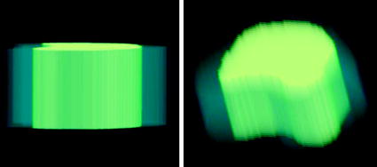
.Fig. 13
The shape model is shown in 3D (when propagating 2D shape model into 3D). The outer volume represents the variability region, the inner volume represents the object region
2.4.4 Initial Segmentation
To estimate the initial labeling  , the ICM method which integrates the intensity and spatial interaction information is used. It should be noted that the shape model has not been used in this process. The initial segmented region is used to obtain the SDF representation which is required in the registration process. An example of the initial labeling is shown in Fig. 14. The method has acceptable results, because a relatively large amount of pedicles and ribs are separated from the vertebral body. It should be noted that there may still some portion of pedicles and ribs which could not be separated. Between Fig. 14d, e, there is a shape registration process which is shown in Figs. 15 and 16.
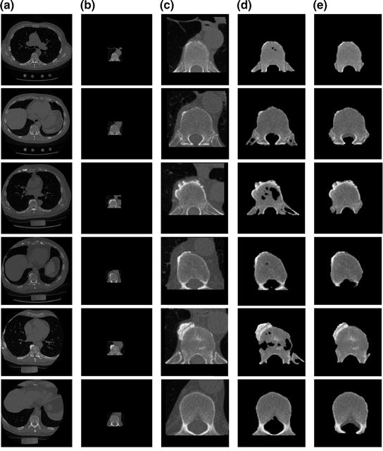
, the ICM method which integrates the intensity and spatial interaction information is used. It should be noted that the shape model has not been used in this process. The initial segmented region is used to obtain the SDF representation which is required in the registration process. An example of the initial labeling is shown in Fig. 14. The method has acceptable results, because a relatively large amount of pedicles and ribs are separated from the vertebral body. It should be noted that there may still some portion of pedicles and ribs which could not be separated. Between Fig. 14d, e, there is a shape registration process which is shown in Figs. 15 and 16.Fig. 14
An example of the initial labeling. a Original CT images. b Detection of the VB region and refinement. c The cropped VB region. d The initial labeling,  using only the intensity and spatial interaction models. e The final segmentation using three models
using only the intensity and spatial interaction models. e The final segmentation using three models
Fig. 15
Embedding the shape model to the image domain and the final segmentation. (i) A CT data after the extraction of spinal cord. (ii) Shape model initialization (the blue color show the outer surface of the variability region  ). The contour
  is placed equally in every slice using the obtained ROI. (iii) Embedding the shape model to the image domain. (iv) Final segmentation using three models: The intensity, spatial interaction, and shape information. Images and results are shown in the (a) sagittal, (b) coronal, and (c) axial views
). The contour is placed equally in every slice using the obtained ROI. (iii) Embedding the shape model to the image domain. (iv) Final segmentation using three models: The intensity, spatial interaction, and shape information. Images and results are shown in the (a) sagittal, (b) coronal, and (c) axial views
Fig. 16
Embedding the shape model to the image domain and the final segmentation. (i) A CT data after the extraction of spinal cord. (ii) Shape model initialization (the blue color show the outer surface of the variability region  ). The contour
  is placed equally in every slice using the obtained ROI. (iii) Embedding the shape model to the image domain. (iv) Final segmentation using three models: The intensity, spatial interaction, and shape information. Images and results are shown in the (a) sagittal, (b) coronal, and (c) axial views
). The contour is placed equally in every slice using the obtained ROI. (iii) Embedding the shape model to the image domain. (iv) Final segmentation using three models: The intensity, spatial interaction, and shape information. Images and results are shown in the (a) sagittal, (b) coronal, and (c) axial views2.4.5 Embedding the Shape Model
To use the shape prior in the segmentation process,  and the shape prior are required to be registered. The shape model has a variability region as shown in Fig. 12a. The outer contour is represented as
  . In the registration process,
  and
and  will be the source and target information, respectively. The registration step is done in 2D slice by slice since the shape model can deform locally independently from other slices. This approach gives deformation flexibility between each slices which stocks in z-axis. The transformation has 4 parameters such as
  ,
,  (for scale,
  ), and
  ,
,  (for translation,
  ). It should be noted that the rotation is not necessary in the method since the registration is done slice by slice; and the VB does not show important rotational variation in the axial axes. Let us define the transformation result by
  that is obtained by applying a transformation
  to a given contour/surface
  . In this case,
  and
and  correspond to
  and
and  , respectively. The transformation can be written for any point
  in the space as
  . Now consider
  and
and  .
.
and the shape prior are required to be registered. The shape model has a variability region as shown in Fig. 12a. The outer contour is represented as . In the registration process, and will be the source and target information, respectively. The registration step is done in 2D slice by slice since the shape model can deform locally independently from other slices. This approach gives deformation flexibility between each slices which stocks in z-axis. The transformation has 4 parameters such as , (for scale, ), and , (for translation, ). It should be noted that the rotation is not necessary in the method since the registration is done slice by slice; and the VB does not show important rotational variation in the axial axes. Let us define the transformation result by that is obtained by applying a transformation to a given contour/surface . In this case, and correspond to and , respectively. The transformation can be written for any point in the space as . Now consider and .The registration of the shape model and testing image is done as follows:

(i)
First, the average of the position factor ( ) and scale factor (
 ) are obtained using the following equations
![$$ \mu^{{{\mathbf{f}}^{ * } }} = \left[ {\begin{array}{*{20}c} {\mu_{x}^{{{\mathbf{f}}^{ * } }} } & {\mu_{y}^{{{\mathbf{f}}^{ * } }} } \\ \end{array} } \right] = \left[ {\begin{array}{*{20}c} {\frac{{\sum\nolimits_{\Upomega } {xH( - \phi_{{{\mathbf{f}}^{ *} }} ({\mathbf{x))}}} }}{{\sum\nolimits_{\Upomega } {H( - \phi_{{{\mathbf{f}}^{ *} }} ({\mathbf{x))}}} }}} & {\frac{{\sum\nolimits_{\Upomega } {yH( - \phi_{{{\mathbf{f}}^{ *} }} ({\mathbf{x))}}} }}{{\sum\nolimits_{\Upomega } {H( - \phi_{{{\mathbf{f}}^{ *} }} ({\mathbf{x))}}} }}} \\ \end{array} } \right]^{T} , $$](/wp-content/uploads/2016/12/A312884_1_En_13_Chapter_Equ21.gif)
![$$ \sigma^{{{\mathbf{f}}^{ * } }} = \left[ {\begin{array}{*{20}c} {(\sigma_{x}^{{{\mathbf{f}}^{ * } }} )^{2} } & {(\sigma_{y}^{{{\mathbf{f}}^{ * } }} )^{2} } \\ \end{array} } \right] = \left[ {\begin{array}{*{20}c} {\frac{{\sum\nolimits_{\Upomega } {(x - \mu_{x}^{{{\mathbf{f}}^{ * } }} )^{2} H( - \phi_{{{\mathbf{f}}^{ * } }} ({\mathbf{x}}\text{))}} }}{{\sum\nolimits_{\Upomega } {H( - \phi_{{{\mathbf{f}}^{ * } }} ({\mathbf{x}}\text{))}} }}} & {\frac{{\sum\nolimits_{\Upomega } {(y - \mu_{y}^{{{\mathbf{f}}^{ * } }} )^{2} H( - \phi_{{{\mathbf{f}}^{ * } }} ({\mathbf{x}}\text{))}} }}{{\sum\nolimits_{\Upomega } {H( - \phi_{{{\mathbf{f}}^{ * } }} ({\mathbf{x}}\text{))}} }}} \\ \end{array} } \right]^{T} . $$](/wp-content/uploads/2016/12/A312884_1_En_13_Chapter_Equ22.gif)
) and scale factor () are obtained using the following equations(21)
(22)
(ii)
Get Clinical Tree app for offline access
Obtain the transformation parameters ( ) for the shape model,
  , as
, as
) for the shape model, , as![$$ {\mathbf{Tr}} = \left[ {\begin{array}{*{20}c} {t_{x} } & {t_{y} } \\ \end{array} } \right]^{T} = \left[ {\begin{array}{*{20}c} {\mu_{x}^{{{\mathbf{f}}^{ * } }} - \frac{{\sum\nolimits_{\Upomega } {xH( - \phi_{{\mathbf{J}}} ({\mathbf{x))}}} }}{{\sum\nolimits_{\Upomega } {H( - \phi_{{\mathbf{J}}} ({\mathbf{x))}}} }}} & {\mu_{y}^{{{\mathbf{f}}^{ * } }} - \frac{{\sum\nolimits_{\Upomega } {yH( - \phi_{{\mathbf{J}}} ({\mathbf{x))}}} }}{{\sum\nolimits_{\Upomega } {H( - \phi_{{\mathbf{J}}} ({\mathbf{x))}}} }}} \\ \end{array} } \right]^{T} , $$](/wp-content/uploads/2016/12/A312884_1_En_13_Chapter_Equ23.gif)